Time Series Analysis

Methods for Real-World Forecasting

Nithin M

Jan 4, 2026

Introduction

• What is time series?
• Examples of time series data
• Why study time series?

• ordered collection of observations; usually equally spaced over time
• mainly to understand the data generating process, forecasting of future values
• special because of autocorrelation among two observations

Components of time series

A time series can be decomposed into 4 components

1. Trend
   • long pattern of the series
   • positive or negative
2. Seasonal
   • regular fluctuations in a specific frequency
3. Cyclical
   • up- down movement over longer periods
   • typical business cycles in macroeconomics
4. Irregular
   • Unpredictable component

Working with R

## Data we use is the inbuilt "AirPassengers" data
plot(AirPassengers)

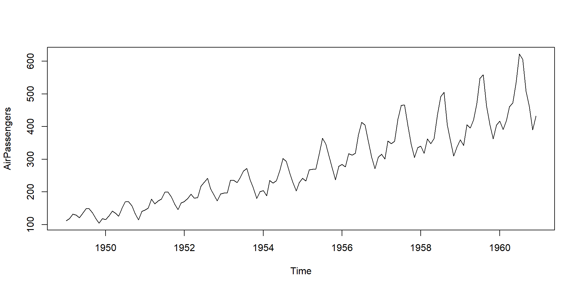
Time series plot of air passengers data

Working with R

plot(decompose(AirPassengers))

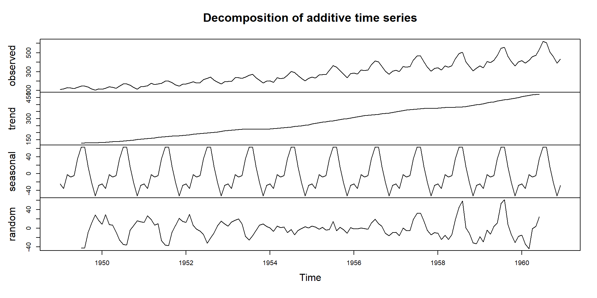
Time series decomposition of air passengers data

Stochastic Process

• a collection of time indexed random variables
• randomness
• time series is actually a realization from certain stochastic process
• stationary and non-stationary process

• \(y(\omega,t)\)
• remeber the bell shape from edx
• cannot be accurately predicted

Stationary Stochastic Process

a discrete stochastic series is stationary if \[\begin{equation} \begin{aligned} &E\left(y_{t}\right)=\mu \\ &E\left(y_{t}-\mu\right)^{2}=\sigma^{2} \\ &E\left[\left(y_{t}-\mu\right)\left(y_{t+k}-\mu\right)\right]=r_{k} \end{aligned} \end{equation}\]

• mention strong form of stationarity
• join distribution is time invariant

White Noise Process

• sequence of uncorrelated random variables from a fixed distribution
• i.i.d

\[\begin{equation} \begin{aligned} &E\left(y_{t}\right)=\mu=0 \\ &E\left(y_{t}-\mu\right)^{2}=Var(y_t)=\sigma_{\mu}^{2} \end{aligned} \end{equation}\]

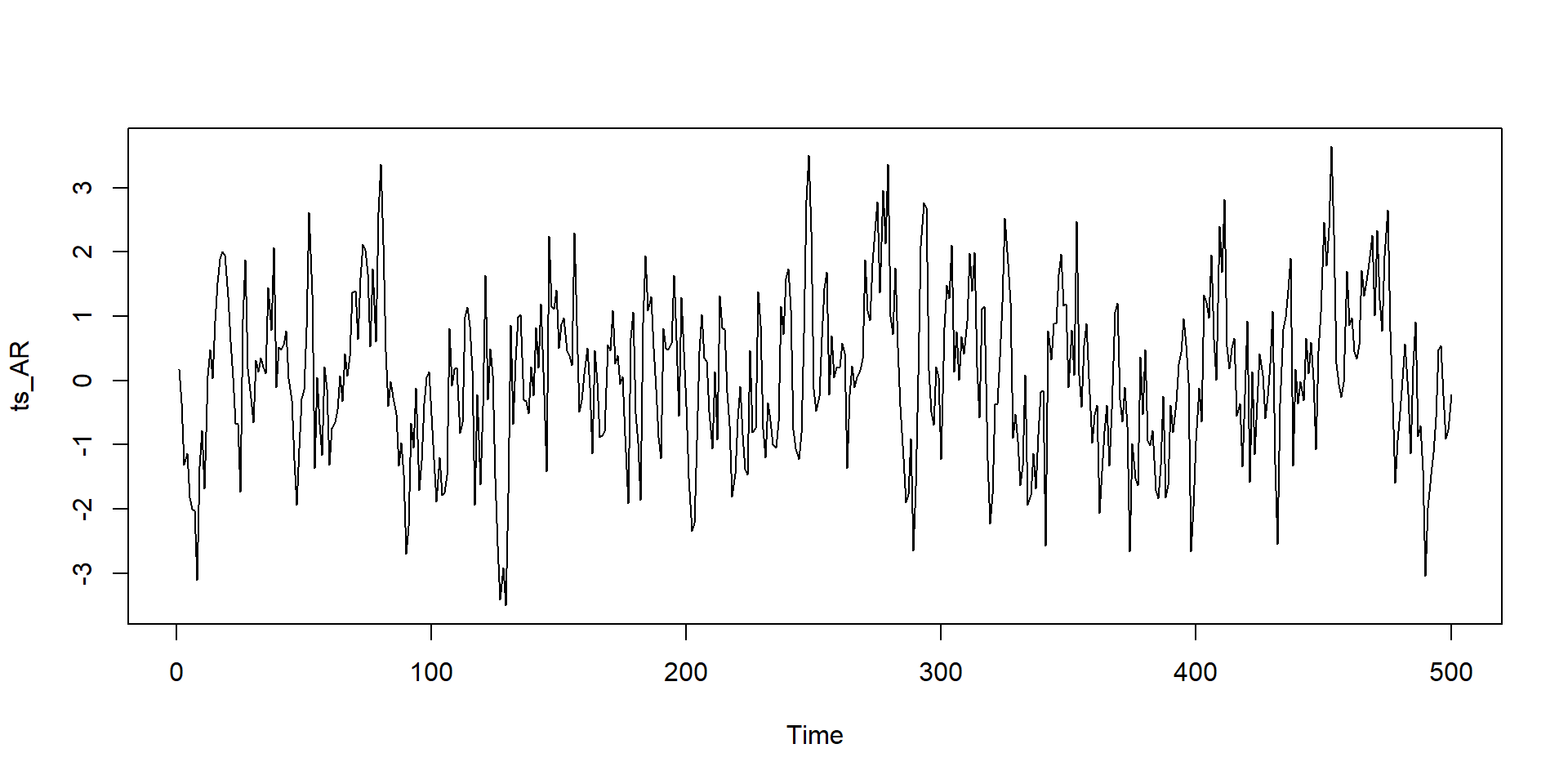
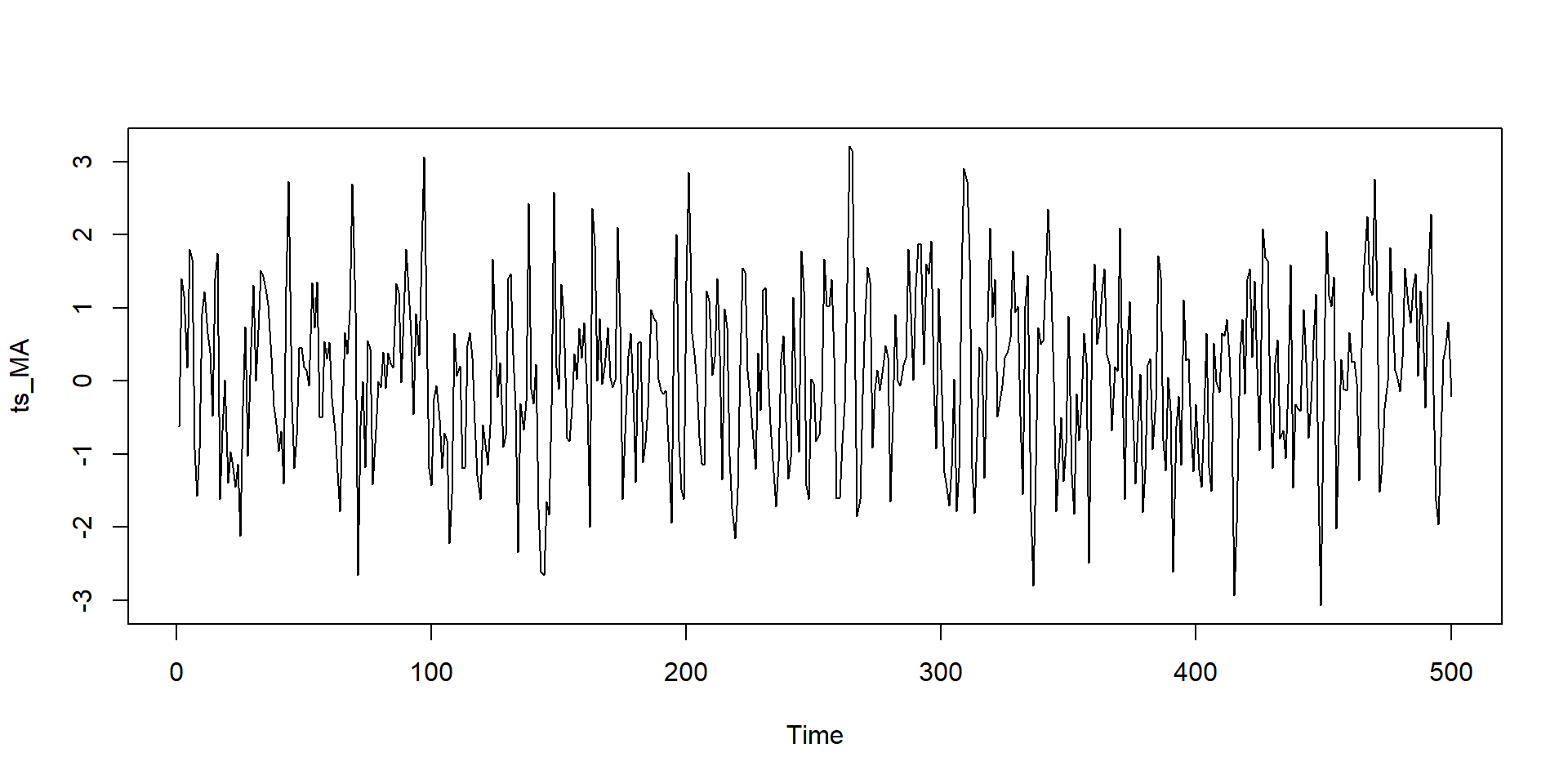
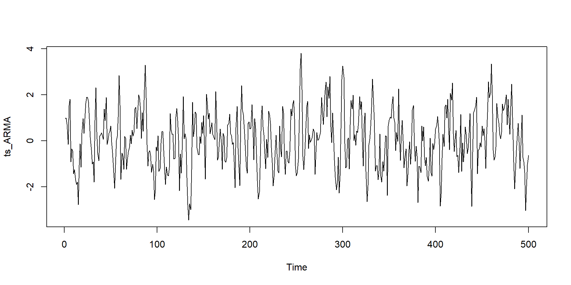
Simulation of Stationary process

• Basic Plot
• XTS package

# purely random process with mean 0 and standard deviation 1
eps <- rnorm(100, mean = 0, sd = 1)
mu <- 2 # the constant mean
# The process
x_t <-mu+ eps

#Conversion to time series
x_t_ts<-ts(x_t, start = c(1990,1),frequency = 12)

x_t_ts

           Jan       Feb       Mar       Apr       May       Jun       Jul
1990 2.8020683 2.9212619 1.5770886 1.9989418 2.7409393 0.3056378 0.1948141
1991 0.9449564 1.3329852 2.4422355 3.7253519 2.7242018 1.6829168 2.2863954
1992 2.7568201 0.8296221 2.6016036 2.0512058 2.3952448 1.7532820 2.4596890
1993 1.9994651 1.6146232 0.8998874 1.6849335 2.0541027 1.5258560 0.3085585
1994 0.3601174 1.6095626 2.9820113 2.3244252 0.5675891 1.4373680 1.4970988
1995 2.6458915 1.1860944 3.3795775 3.3793787 2.2896724 3.9349686 1.8168275
1996 1.7202123 2.2061306 2.1530900 0.4199460 1.6099486 1.0203606 2.2224175
1997 0.9356408 3.1818449 2.2896916 2.9076898 2.4721116 2.7782292 2.0620099
1998 1.3474332 1.9972262 1.7807013 2.1818773                              
           Aug       Sep       Oct       Nov       Dec
1990 2.7699693 1.9840060 1.9207495 3.1591849 3.0527548
1991 1.7277774 1.7189432 3.5322217 1.9321485 2.1946392
1992 0.6452703 1.9654789 3.0813508 2.3363887 1.4197945
1993 1.1028343 0.3825236 0.8409247 1.0223992 1.6148691
1994 2.4919466 1.1360051 2.1254101 0.5343036 1.7909002
1995 1.6267527 3.5949415 2.2261651 3.0460791 4.6742249
1996 2.5571245 1.2519367 2.1954782 2.3655836 1.0772995
1997 0.4591330 2.1296115 1.2022569 1.1535417 2.6936724
1998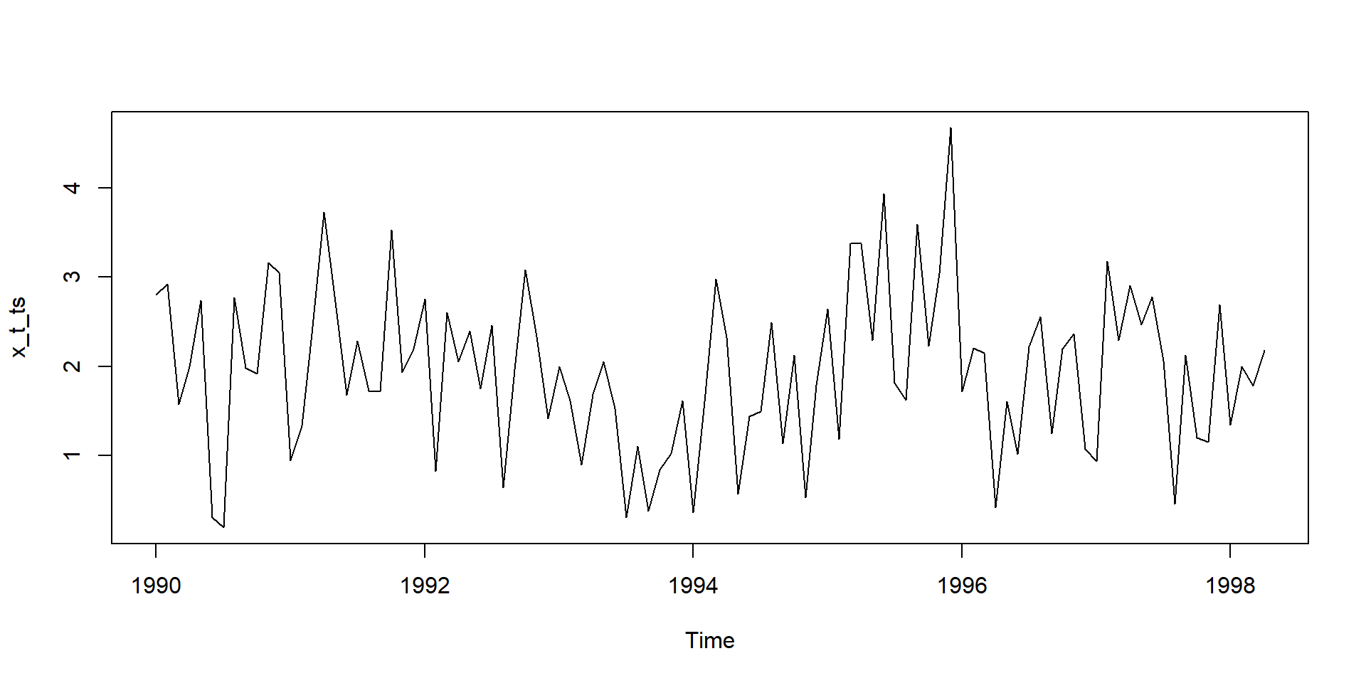                                                  

plot(x_t_ts)

# purely random process with mean 0 and standard deviation 1
eps <- rnorm(100, mean = 0, sd = 1)
mu <- 2 # the constant mean
# The process
x_t <-mu+ eps

#Conversion to time series
library(xts)
xt_xts<-as.xts(x_t_ts)
xt_xts

              [,1]
Jan 1990 2.8020683
Feb 1990 2.9212619
Mar 1990 1.5770886
Apr 1990 1.9989418
May 1990 2.7409393
Jun 1990 0.3056378
Jul 1990 0.1948141
Aug 1990 2.7699693
Sep 1990 1.9840060
Oct 1990 1.9207495
Nov 1990 3.1591849
Dec 1990 3.0527548
Jan 1991 0.9449564
Feb 1991 1.3329852
Mar 1991 2.4422355
Apr 1991 3.7253519
May 1991 2.7242018
Jun 1991 1.6829168
Jul 1991 2.2863954
Aug 1991 1.7277774
Sep 1991 1.7189432
Oct 1991 3.5322217
Nov 1991 1.9321485
Dec 1991 2.1946392
Jan 1992 2.7568201
Feb 1992 0.8296221
Mar 1992 2.6016036
Apr 1992 2.0512058
May 1992 2.3952448
Jun 1992 1.7532820
Jul 1992 2.4596890
Aug 1992 0.6452703
Sep 1992 1.9654789
Oct 1992 3.0813508
Nov 1992 2.3363887
Dec 1992 1.4197945
Jan 1993 1.9994651
Feb 1993 1.6146232
Mar 1993 0.8998874
Apr 1993 1.6849335
May 1993 2.0541027
Jun 1993 1.5258560
Jul 1993 0.3085585
Aug 1993 1.1028343
Sep 1993 0.3825236
Oct 1993 0.8409247
Nov 1993 1.0223992
Dec 1993 1.6148691
Jan 1994 0.3601174
Feb 1994 1.6095626
Mar 1994 2.9820113
Apr 1994 2.3244252
May 1994 0.5675891
Jun 1994 1.4373680
Jul 1994 1.4970988
Aug 1994 2.4919466
Sep 1994 1.1360051
Oct 1994 2.1254101
Nov 1994 0.5343036
Dec 1994 1.7909002
Jan 1995 2.6458915
Feb 1995 1.1860944
Mar 1995 3.3795775
Apr 1995 3.3793787
May 1995 2.2896724
Jun 1995 3.9349686
Jul 1995 1.8168275
Aug 1995 1.6267527
Sep 1995 3.5949415
Oct 1995 2.2261651
Nov 1995 3.0460791
Dec 1995 4.6742249
Jan 1996 1.7202123
Feb 1996 2.2061306
Mar 1996 2.1530900
Apr 1996 0.4199460
May 1996 1.6099486
Jun 1996 1.0203606
Jul 1996 2.2224175
Aug 1996 2.5571245
Sep 1996 1.2519367
Oct 1996 2.1954782
Nov 1996 2.3655836
Dec 1996 1.0772995
Jan 1997 0.9356408
Feb 1997 3.1818449
Mar 1997 2.2896916
Apr 1997 2.9076898
May 1997 2.4721116
Jun 1997 2.7782292
Jul 1997 2.0620099
Aug 1997 0.4591330
Sep 1997 2.1296115
Oct 1997 1.2022569
Nov 1997 1.1535417
Dec 1997 2.6936724
Jan 1998 1.3474332
Feb 1998 1.9972262
Mar 1998 1.7807013
Apr 1998 2.1818773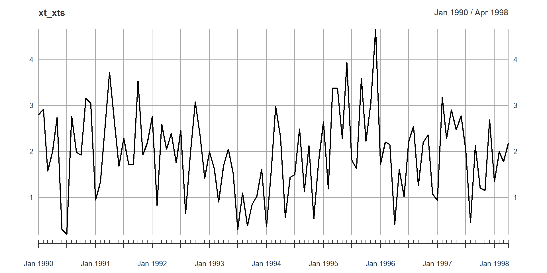

plot(xt_xts)

White noise process in R

• Using base R
• using stats package

plot(rnorm(100),type="l")

white_noise<- arima.sim(model = list(order = c(0, 0, 0)), n = 100)

# Plot the WN observations
ts.plot(white_noise)

Autocorrelation and Autocovariance Functions

• both as functions of only time differences \(|t-s|\)

• Autocovariance \[\begin{equation} \gamma_{k}=\operatorname{Cov}\left(Z_{t}, Z_{t+k}\right)=E\left(Z_{t}-\mu\right)\left(Z_{t+k}-\mu\right) \end{equation}\]

• Autocorrelation Function (ACF) \[\begin{equation} \rho_{k}=\frac{\operatorname{Cov}\left(Z_{t}, Z_{f+k}\right)}{\sqrt{\operatorname{Var}\left(Z_{f}\right)} \sqrt{\operatorname{Var}\left(Z_{t+k}\right)}}=\frac{\gamma_{k}}{\gamma_{0}} \end{equation}\]

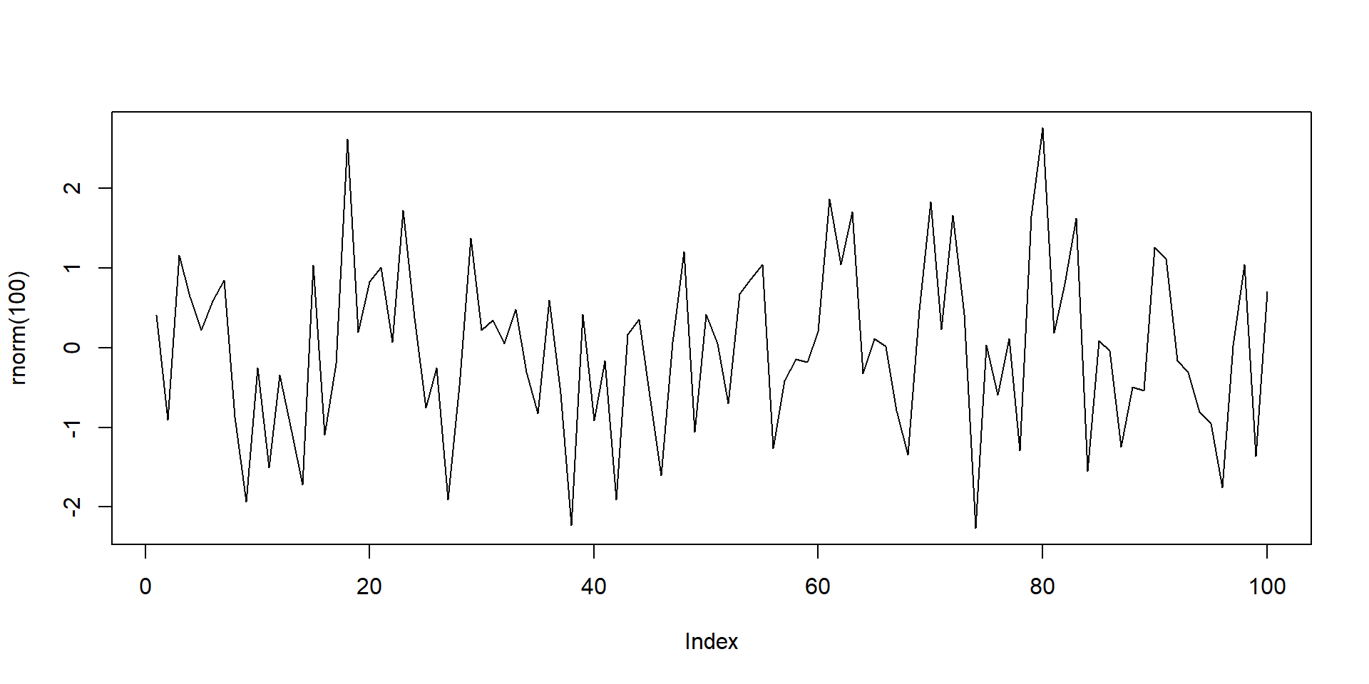
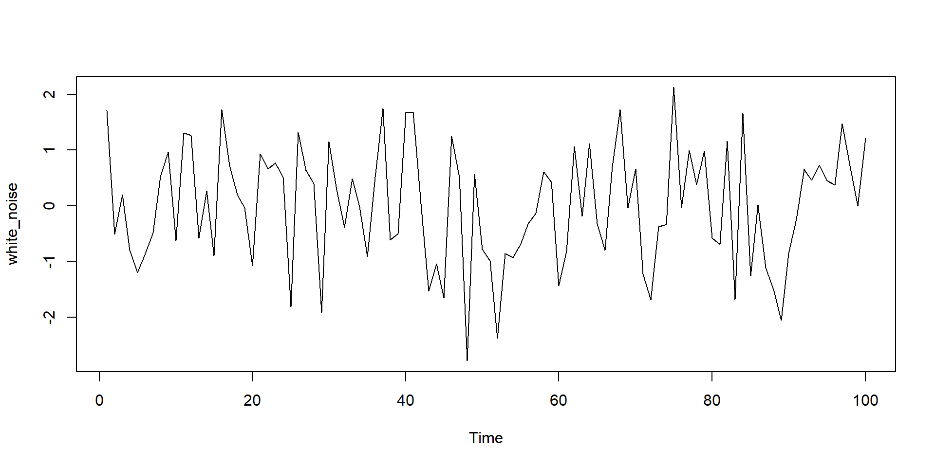
Implementation in R

• ACF Table
• ACF plot

library(forecast)
ggAcf(AirPassengers,lag.max = 10,plot = F)

Autocorrelations of series 'AirPassengers', by lag

    0     1     2     3     4     5     6     7     8     9    10 
1.000 0.948 0.876 0.807 0.753 0.714 0.682 0.663 0.656 0.671 0.703 

ggAcf(co2,lag.max = 10,plot = T)+ggplot2::theme_bw()

Univariate Time Series

Stationary Time Series

• 3 important process

  1. Moving Average (MA) \[ y_{t}=\mu+u_{t}+\phi_{1} u_{t-1}+\phi_{2} u_{t-2}+\ldots+\phi_{t} u_{t} \]

  2. Autoregressive (AR) \[ y_{t}=a+b_{1} y_{t-1}+b_{2} y_{t-2}+\ldots .+b_{p} y_{t}+\varepsilon_{t} \]

  3. ARMA Process \[ \begin{aligned} &y_{t}=a+b_{1}y_{t-1}+b_{2}y_{t-2}+\ldots+b_{p}y_{t-p} \\ &+u_{t}+\phi_{1} u_{t-1}+\phi_{2} u_{t-2}+\ldots+\phi_{q} u_{t-q} \end{aligned} \]

Steps in analysis of stationary series

1. Identification
   • visual inspection

• AR(1) process
• MA (1) process
• ARMA process

set.seed(123)
ts_AR <- arima.sim(n = 500, list(ar = 0.7))
plot(ts_AR)

set.seed(123)
ts_MA<-arima.sim(n = 500, list(ma = 0.7))
plot(ts_MA)

set.seed(123)
ts_ARMA<-arima.sim(n = 500, list(ar=0.5,ma = 0.3))
plot(ts_ARMA)

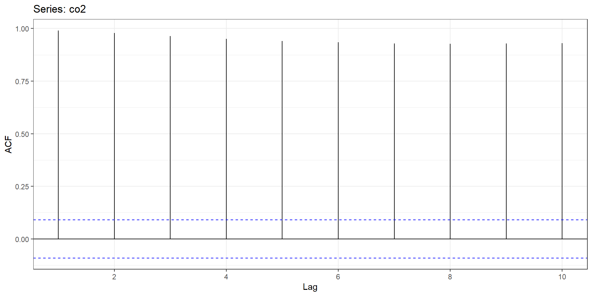
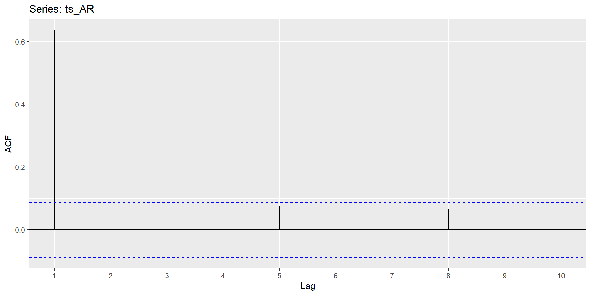
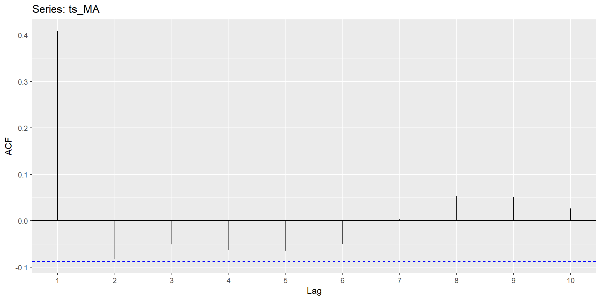
Formal identification

Autocorrelation Function

• AR(1) process
• MA(1) process

ggAcf(ts_AR,lag.max=10)

ggAcf(ts_MA,lag.max=10)

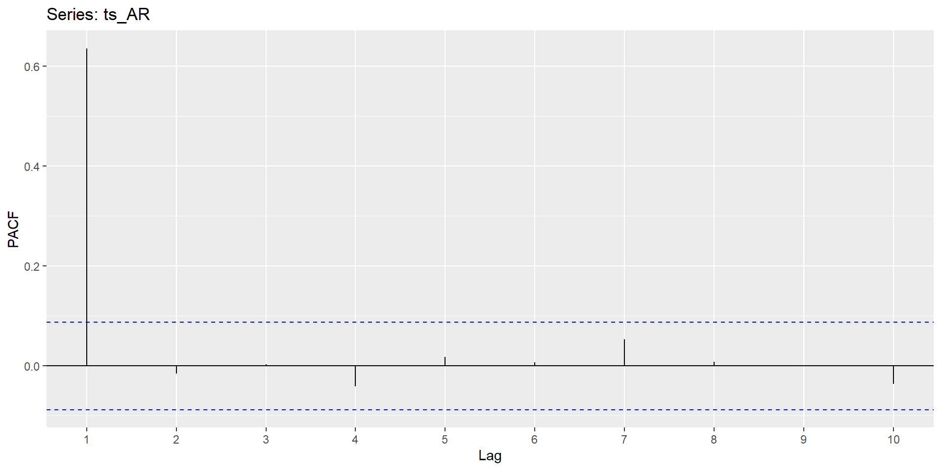
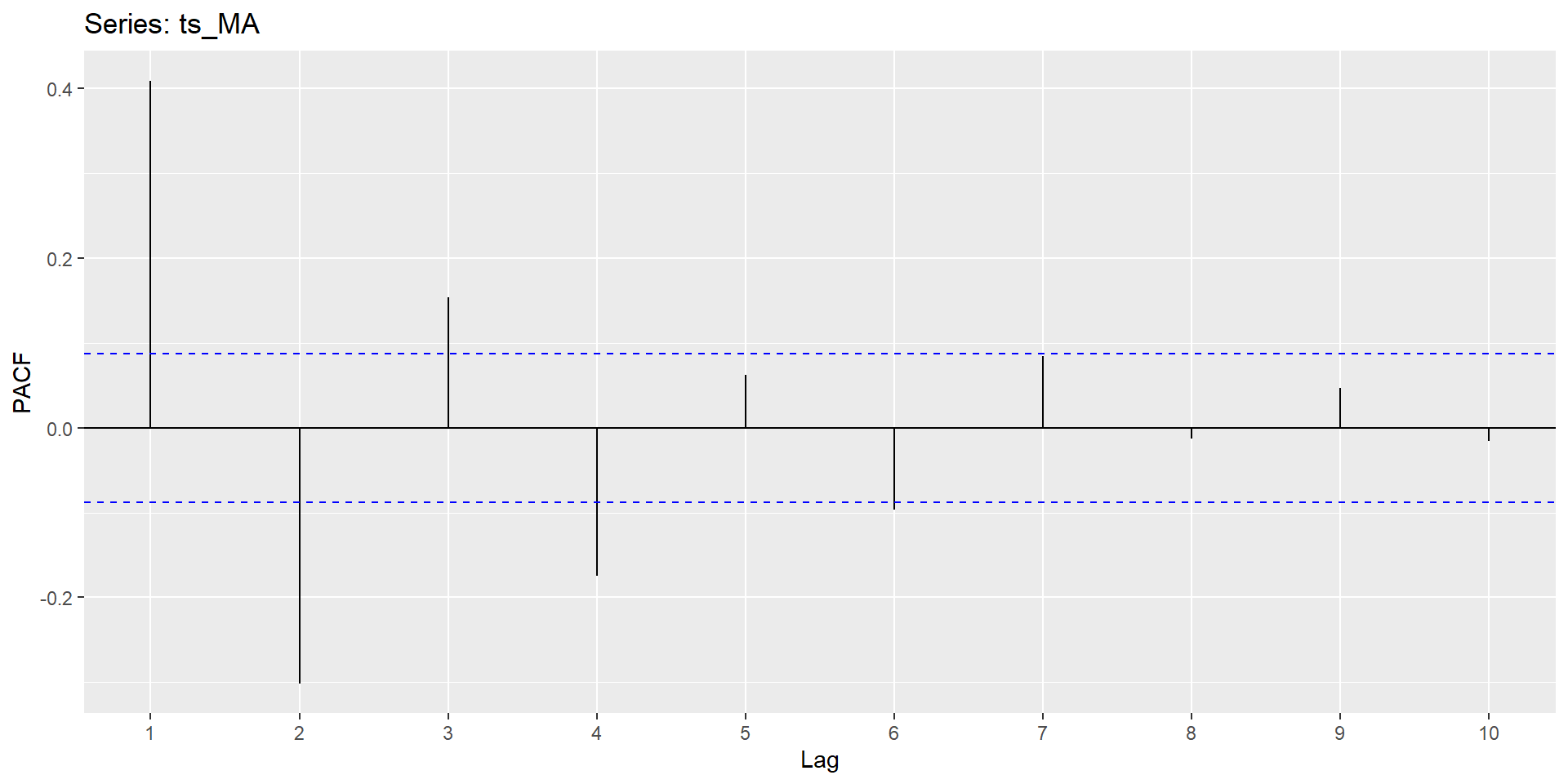
Formal identification (Cont.)

Partial Autocorrelation Function

• AR(1) process
• MA(1) process

ggPacf(ts_AR,lag.max=10)

ggPacf(ts_MA,lag.max=10)

The \(p^{\text {th }}\) partial autcorrelation is the \(p^{\text {th }}\) coefficient of linear regression of \(y_{+}\)on its lags up to \(p\) :

Formal identification (Cont.)

Summary of Patterns to look for

Non-stationary Process

• A variable \(y_t\) is non-stationary, if it has time varying mean or time varying variance or both
  
• There is no mean reversion
• 3 types
  1. Random Walk without drift
  2. Random walk with drift
  3. Random walk with drift and deterministic trend

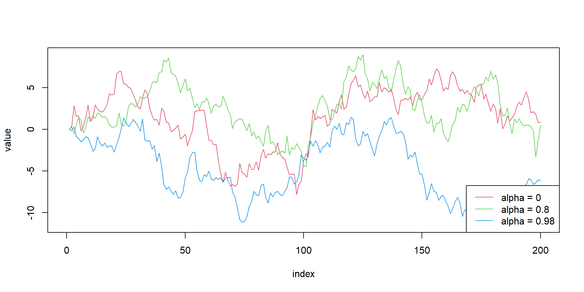
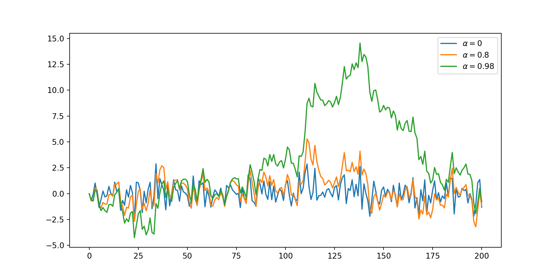
Random walk - Simulation

• R
• Python

# Set-up

alphas<-c(0,0.8,0.98)
obs<-array(0,200)
list_rw<-list()
for(m in 1:3){
for(i in alphas){
  for (j in 2:length(obs) ){
    obs[j]=i*obs[j-1]+rnorm(1)
  }
}
  list_rw[[m]]<-obs
  
}


#limit calculation
ymax=max(sapply(list_rw,max))
ymin=min(sapply(list_rw,min))

#empty plot
plot(NULL, xlab = "index", ylab = "value", xlim = c(0, length(obs)), ylim = c(ymin,ymax))

#plot lines
for(i in seq_along(list_rw)){
  lines(x=1:200,y=list_rw[[i]], type = "l", lty = 1, col = i +1 )
}

# Legends
legend("bottomright", legend = paste0("alpha = ", alphas), lty = 1, col = 1 + seq_along(alphas))

import numpy as np
import matplotlib.pyplot as plt

α=[0,0.8,0.98]
T = 200
x = [0]*(T+1)
ϵ=np.random.randn(T)
for j in α:
    x[0] = 0
    for i in range(T):
         x[i+1]=j *x[i]+ϵ[i]
    plt.plot(x, label=f'$\\alpha = {j}$')

plt.legend()
plt.show()

Integrated Stochastic Process

• RWP is non-stationary but its first difference is stationary \[\begin{equation} \begin{aligned} &y_{t}=y_{t-1}+\varepsilon_{t} \\ &\Delta y_{t}=\varepsilon_{t} \end{aligned} \end{equation}\]

• \(y_t\) is said to be integrated of order 1 (\(y_{t} \sim I(1)\))

• simillarly, \(y_t \sim I(2)\) if \(\Delta^{2} y_{t}=\varepsilon_{t}\)

introduce lag operator

\(Ly_t= y_{t-1}\)

\[ y_{t}^{\prime}=y_{t}-y_{t-1}=y_{t}-L y_{t}=(1-L) y_{t} \]

Consequences of Non-Stationarity

• Shocks do not “die” out
• Statistical consequences
  • Non normal distribution of test statistics
  • Bias in AR coefficients
  • Poor forecasts
  • Spurious Regression

Testing for Non-Stationarity

• Unit root problem
• Conventional Unit root tests
  • DF test
  • ADF test
  • PP test
  • DF GLS test
• Unit root with structural breaks
• KPSS stationarity test

DF test, errors are white noise while in ADF we allow for autocorrelation in PP errors are ARMA - PP based on aymptotic properties

Where do we go from here??

Advanced Topics

• ARIMA models
• Modelling Volatility- ARCH/GARCH class of models
• Multivariate time series - VAR/VECM
• Non-linear time series - TAR/SETAR, MRS, KF

Practical Time Series in R

Loading Data

• a R dataframe is not a time series object by defauls
• need packages like xts, zoo, tsibble etc., to handle time series data

# A tibble: 12 × 2
   date       value
   <date>     <int>
 1 2020-01-01  3821
 2 2020-02-01  3262
 3 2020-03-01  3219
 4 2020-04-01  4039
 5 2020-05-01  3004
 6 2020-06-01  3151
 7 2020-07-01  4903
 8 2020-08-01  3695
 9 2020-09-01  4138
10 2020-10-01  3681
11 2020-11-01  4568
12 2020-12-01  3115

• observe the date column; not a time series object yet
• this is just a regular dataframe with a date column

Converting to time series object

• Default tsibble conversion
• adjusting frequency

library(tsibble)
ts_data <- table %>%
  as_tsibble(index = date)
print(ts_data)

# A tsibble: 12 x 2 [1D]
   date       value
   <date>     <int>
 1 2020-01-01  3821
 2 2020-02-01  3262
 3 2020-03-01  3219
 4 2020-04-01  4039
 5 2020-05-01  3004
 6 2020-06-01  3151
 7 2020-07-01  4903
 8 2020-08-01  3695
 9 2020-09-01  4138
10 2020-10-01  3681
11 2020-11-01  4568
12 2020-12-01  3115

library(dplyr)
library(lubridate)
ts_data <- table %>%
  mutate(date = yearmonth(date)) %>%
  as_tsibble(index = date)
print(ts_data)

# A tsibble: 12 x 2 [1M]
       date value
      <mth> <int>
 1 2020 Jan  3821
 2 2020 Feb  3262
 3 2020 Mar  3219
 4 2020 Apr  4039
 5 2020 May  3004
 6 2020 Jun  3151
 7 2020 Jul  4903
 8 2020 Aug  3695
 9 2020 Sep  4138
10 2020 Oct  3681
11 2020 Nov  4568
12 2020 Dec  3115

Some Data

Load the data gh_data.csv - some cleaning - pivoting and making tidy data - converting to tsibble - gaps in data

Now load the sales.csv

• handling gaps in the data

Working Dates and Time

• conversion of date-time formats
• date arithmetic
• parse_date_time from lubridate package

Time series features

• calender features
• lagged features
• differenced features
• visualisation

Exploratory Time Series Analysis

Why Exploratory Analysis Matters

• Pattern Discovery: Uncover seasonal patterns, trends, and cycles that drive your time series.

• Anomaly Detection: Identify outliers and unusual events that might distort your model.

• Model Selection: Understand the type of forecasting method that might work best for your data.

• Business Insights: For financial time series data you can transform raw numbers into actionable intelligence.

• Data Quality: Catch any data issues before they compromise your analysis.

Visual Exploration

• ggplot2 package for visualisation
• autoplot function from feasts package

Exploring Patterns

• Trend analysis
• Seasonal patterns
• Cyclical patterns
• Irregular components
• AR, MA, ACF, PACF plots

Forecasting

Forecasting Methods

use of fable package for forecasting

• Naive Forecasting
• Mean Forecasting
• Seasonal Naive Forecasting
• ETS
• ARIMA
• SARIMA

Putting it all together

• load `gh_cocoa.csv’ data
• fit some models

Let us have fun with time series!!

Thank You!