Lecture 12: Foreign Exchange Market — Instruments and Policy

Econ 2203 | International Trade and Policy in Agriculture

Nithin M

Department of Development Economics

2026-07-11

Forex Market: Exchange Rate Systems and Open Economy Macro

From exchange rate regimes to the Mundell-Fleming model — how monetary and fiscal policy interact with the exchange rate, and what this means for agricultural exporters and importers.

Recap (Lecture 11): key equations

\[e = \frac{\text{domestic currency}}{\text{foreign currency}}\]

  • Absolute PPP: \(e = \frac{P_d}{P_f}\)
  • Relative PPP: \(\frac{\Delta e}{e} = \pi_d - \pi_f\)
  • UIP: \(i = i^* + \frac{E(e_{t+1}) - e_t}{e_t}\)

Recap: India numerical context (illustrative)

  • INR/USD spot ≈ ₹83.5/$
  • India CPI inflation ≈ 5–6%; US ≈ 2–3%
  • Relative PPP → ~3–4% annual INR depreciation
  • Repo rate ≈ 6.5%; Fed funds ≈ 5.25–5.5%

Today (Lecture 12): what we add

  • Exchange rate regimes (fixed vs float vs managed)
  • Mundell–Fleming: policy under different regimes
  • RBI intervention and reserves logic
  • Forward markets + hedging for agri trade

Exchange Rate Systems (I): Free Float and Managed Float

System Description India Relevance
Free float Market determines exchange rate; central bank does not intervene USA, UK, Eurozone — India’s major trading partners operate under this system
Managed float CB intervenes to smooth volatility but does not target a specific level India’s current system (since 1993 post-LERMS); RBI smooths but allows gradual adjustment

India’s choice: Managed float since 1993 (post-LERMS). RBI intervenes to smooth but does not target a specific level. This preserves monetary policy independence while preventing destabilising volatility.

Exchange Rate Systems (II): Fixed and Intermediate Regimes

System Description India Relevance
Crawling peg Regular small, pre-announced adjustments to the peg Chile historically; some SAARC neighbours use variants
Fixed/pegged CB maintains exchange rate at a predetermined target using reserves Gulf states (USD peg); pre-1991 India maintained a de facto fixed rate
Currency board 100% foreign reserve backing for domestic currency at fixed rate Argentina 1991–2001 (collapsed); Hong Kong (ongoing)
Currency union Single shared currency across multiple countries Eurozone; CFA Franc zone in West/Central Africa

Historical lesson for India: India maintained a de facto fixed rate through the 1980s. By 1991: BoP crisis forced a 44% devaluation. Post-crisis shift to managed float was the correct policy response.

Fixed exchange rate: pros and cons (agriculture)

  • Predictable rate helps long contracts (exports/imports)
  • Can discipline inflation (money creation constrained)
  • Risk of overvaluation → sudden crisis + forced devaluation
  • Monetary policy autonomy is limited
  • Requires reserves to defend the peg

Flexible exchange rate: pros and cons (agriculture)

  • Automatic adjustment via depreciation/appreciation
  • Monetary policy has more room
  • Volatility creates pricing risk for traders
  • Depreciation raises costs of key imports (oil, fertiliser, edible oils)

Case Study: India’s 1991 Exchange Rate Crisis

India’s 1991 crisis — the case for managed float:

India maintained a de facto fixed rate through the 1980s. By 1991: BoP deficit widened, reserves fell to $1.2B (barely 2 weeks of import cover), credit rating downgraded. India was forced to devalue 44% in two days (July 1–3, 1991). Post-crisis, India adopted the Liberalised Exchange Rate Management System (LERMS) in 1992, transitioning to a managed float by 1993. The lesson: a fixed rate without adequate reserves and fiscal discipline is a crisis waiting to happen.

The Impossible Trinity: Statement and Intuition

Statement: A country CANNOT simultaneously maintain all three of:

  1. 🔒 Fixed exchange rate (\(e = \bar{e}\))
  2. 🌐 Free capital mobility (\(CF\) unconstrained)
  3. 🏦 Independent monetary policy (\(i \neq i^*\))

Mathematical intuition: Under a fixed rate (\(e = \bar{e}\)) and free capital (\(CF\) unconstrained), UIP forces \(i = i^*\). Then monetary policy (\(M\)) cannot change \(i\) independently — any attempt to lower \(i\) below \(i^*\) triggers capital outflow, forcing the CB to sell reserves to defend the peg, which contracts \(M\) back.

\[\{e_{\text{fixed}}\} \cup \{CF_{\text{free}}\} \cup \{MP_{\text{independent}}\}: \text{ choose any TWO}\]

India’s trilemma choice: Managed float (partial exchange rate flexibility) + selective capital controls (FPI restrictions, ECB limits) = partial monetary independence. A pragmatic middle path.

The Impossible Trinity: Country Examples

Country Fixed rate? Free capital? Monetary independence?
USA (free float)
Eurozone ✓ (intra-EU)
China (capital controls)
India (managed float) Partial Partial Partial
Argentina 1991–2001 ✗ → Crisis!

India and the Impossible Trinity

India’s capital account structure:

  • FDI: largely free — automatic route for most sectors
  • FPI (Foreign Portfolio Investment): restricted — SEBI-regulated limits on equity and debt holdings by foreign investors
  • ECB (External Commercial Borrowing): regulated — sector-specific limits, end-use restrictions, all-in cost ceilings

RBI maintains independent monetary policy:

  • Repo rate currently 6.5% (June 2026) despite US Fed at 5.25–5.5%
  • If India fully opened the capital account, carry trade would force UIP: either the rupee would appreciate sharply to equalise returns, OR RBI would have to cut rates to match the US Fed

2013 Taper Tantrum — proof of concept:

When Bernanke signalled Fed tapering (May 2013), capital fled emerging markets. India’s partial capital openness was enough to expose it: rupee fell ₹56 → ₹68 in weeks (-18%). RBI was forced to raise rates sharply to 7.25% and tighten capital controls temporarily. Full capital openness would have made this worse. Selective capital controls preserved room for monetary manoeuvre.

Agricultural angle: Capital account policy affects rupee stability, which directly affects agri export competitiveness and the cost of imported inputs (edible oil, fertiliser). A sudden capital-flight-driven depreciation hurts edible oil importers; a sudden appreciation hurts rice and cotton exporters.

The Mundell-Fleming Model: Open Economy IS-LM

Description: IS-LM extended for the open economy with a Balance of Payments equilibrium condition.

Three equations:

\[IS: Y = C(Y-T) + I(i) + G + NX(e, Y, Y^*)\]

\[LM: \frac{M}{P} = L(i, Y)\]

\[BP: 0 = NX(e, Y, Y^*) + CF(i - i^*)\]

Where:

  • $NX = $ net exports — falls when \(Y\) rises (more imports); rises when \(e\) rises (depreciation makes exports cheaper)
  • $CF = $ capital flows — rises when \(i\) rises relative to world rate \(i^*\)
  • \(BP = 0\) at external balance — the BoP equilibrium condition

BP curve in \((Y, i)\) space: Upward sloping — higher \(Y\) → more imports → BoP deficit → need higher \(i\) to attract offsetting capital inflow.

Capital mobility and BP slope: With high capital mobility, small changes in \(i\) generate large capital flows → BP curve is nearly flat (horizontal at \(i = i^*\) under perfect mobility). With low capital mobility, large changes in \(i\) are needed → BP curve is steep. India: intermediate case, moderate upward slope.

MF Model: Fixed Exchange Rate — Fiscal Policy Effective, Monetary Ineffective

Show R code
# Panel 1: Fiscal expansion under fixed rate (effective)
p_fiscal <- ggplot() +
  geom_segment(aes(x=20, y=12, xend=80, yend=2), color="#012169", linewidth=1.5) +
  annotate("text", x=82, y=2.2, label="IS", size=4, color="#012169") +
  geom_segment(aes(x=32, y=12, xend=92, yend=2), color="#012169", linewidth=1.2, linetype="dashed") +
  annotate("text", x=94, y=2.2, label="IS'", size=4, color="#012169") +
  geom_segment(aes(x=20, y=2, xend=80, yend=12), color="#B9975B", linewidth=1.5) +
  annotate("text", x=82, y=12, label="LM", size=4, color="#B9975B") +
  geom_hline(yintercept=7, linetype="dotdash", color="darkgreen", linewidth=1.2) +
  annotate("text", x=85, y=7.5, label="BP (i=i*)", size=3.5, color="darkgreen") +
  geom_point(aes(x=50, y=7), size=4, color="black") +
  geom_point(aes(x=62, y=7), size=4, color="darkgreen") +
  annotate("text", x=48, y=7.8, label="E1", size=3.5) +
  annotate("text", x=64, y=7.8, label="E2\n(Y rises!)", size=3.2, color="darkgreen") +
  annotate("segment", x=52, y=7, xend=60, yend=7,
           arrow=arrow(length=unit(0.25,"cm")), color="darkgreen") +
  annotate("text", x=56, y=5.8,
           label="G↑ → IS shifts right\nFixed rate: LM adjusts via\nreserve inflow → Y↑",
           size=2.8, color="darkgreen", hjust=0.5) +
  labs(title="Fiscal Expansion (G↑): EFFECTIVE",
       subtitle="Fixed rate + capital mobility: no crowding out",
       x="Output (Y)", y="Interest Rate (i)") +
  coord_cartesian(xlim=c(15,100), ylim=c(0,15)) +
  theme_minimal(base_size=10)

# Panel 2: Monetary expansion under fixed rate (ineffective)
p_monetary <- ggplot() +
  geom_segment(aes(x=20, y=12, xend=80, yend=2), color="#012169", linewidth=1.5) +
  annotate("text", x=82, y=2.2, label="IS", size=4, color="#012169") +
  geom_segment(aes(x=20, y=2, xend=80, yend=12), color="#B9975B", linewidth=1.5) +
  annotate("text", x=82, y=12, label="LM", size=4, color="#B9975B") +
  geom_segment(aes(x=32, y=2, xend=92, yend=12), color="#B9975B", linewidth=1.2, linetype="dashed") +
  annotate("text", x=94, y=12, label="LM'", size=4, color="#B9975B") +
  geom_hline(yintercept=7, linetype="dotdash", color="darkgreen", linewidth=1.2) +
  annotate("text", x=85, y=7.5, label="BP (i=i*)", size=3.5, color="darkgreen") +
  geom_point(aes(x=50, y=7), size=4, color="black") +
  geom_point(aes(x=62, y=4), size=3, color="grey60") +
  annotate("text", x=48, y=7.8, label="E1", size=3.5) +
  annotate("text", x=64, y=3.5, label="E' (temp)", size=3, color="grey60") +
  annotate("segment", x=67, y=6, xend=57, yend=6.5,
           arrow=arrow(length=unit(0.25,"cm")), color="red") +
  annotate("text", x=68, y=6.3,
           label="M↑ → i falls → capital\noutflow → CB sells USD\n→ M contracts back\n→ LM returns to LM!",
           size=2.7, color="red", hjust=0) +
  labs(title="Monetary Expansion (M↑): INEFFECTIVE",
       subtitle="Fixed rate: M expansion fully offset by reserve loss",
       x="Output (Y)", y="Interest Rate (i)") +
  coord_cartesian(xlim=c(15,100), ylim=c(0,15)) +
  theme_minimal(base_size=10)

p_fiscal + p_monetary +
  plot_annotation(
    title="Mundell-Fleming: Fixed Exchange Rate Regime",
    subtitle="Key result: Fiscal policy highly effective; Monetary policy completely ineffective"
  )

Figure 1

Mathematical mechanism — why monetary policy fails under fixed rate:

Under fixed \(e\): \(M\uparrow \Rightarrow i\downarrow \Rightarrow\) capital outflow \(\Rightarrow\) BoP deficit \(\Rightarrow\) CB sells reserves \(\Rightarrow M\) contracts back to original level.

Agricultural policy implication: Under a fixed rate, only government spending (e.g., irrigation subsidies, MSP support operations, fertiliser subsidies) can stimulate the farm economy — not RBI rate cuts. The RBI is powerless to lower borrowing costs for farmers if the exchange rate is pegged.

MF Model: Flexible Exchange Rate — Monetary Effective, Fiscal Crowded Out

Show R code
# Panel 1: Monetary expansion under flexible (effective)
p_mon_flex <- ggplot() +
  geom_segment(aes(x=20, y=12, xend=80, yend=2), color="#012169", linewidth=1.5) +
  annotate("text", x=82, y=2.2, label="IS", size=4, color="#012169") +
  geom_segment(aes(x=32, y=12, xend=92, yend=2), color="#012169", linewidth=1.2, linetype="dashed") +
  annotate("text", x=94, y=2.2, label="IS'", size=4, color="#012169") +
  geom_segment(aes(x=20, y=2, xend=80, yend=12), color="#B9975B", linewidth=1.5) +
  annotate("text", x=82, y=12, label="LM", size=4, color="#B9975B") +
  geom_segment(aes(x=32, y=2, xend=92, yend=12), color="#B9975B", linewidth=1.2, linetype="dashed") +
  annotate("text", x=94, y=12, label="LM'", size=4, color="#B9975B") +
  geom_hline(yintercept=7, linetype="dotdash", color="darkgreen", linewidth=1.2) +
  annotate("text", x=85, y=7.5, label="BP (i=i*)", size=3.5, color="darkgreen") +
  geom_point(aes(x=50, y=7), size=4, color="black") +
  geom_point(aes(x=68, y=7), size=4, color="darkgreen") +
  annotate("text", x=48, y=7.8, label="E1", size=3.5) +
  annotate("text", x=70, y=7.8, label="E2\n(Y rises!)", size=3.2, color="darkgreen") +
  annotate("segment", x=52, y=7, xend=66, yend=7,
           arrow=arrow(length=unit(0.25,"cm")), color="darkgreen") +
  annotate("text", x=56, y=5.3,
           label="M↑ → i↓ → capital outflow\n→ currency depreciates\n→ NX↑ → IS shifts right\n→ Y rises at same i*",
           size=2.7, color="darkgreen", hjust=0.5) +
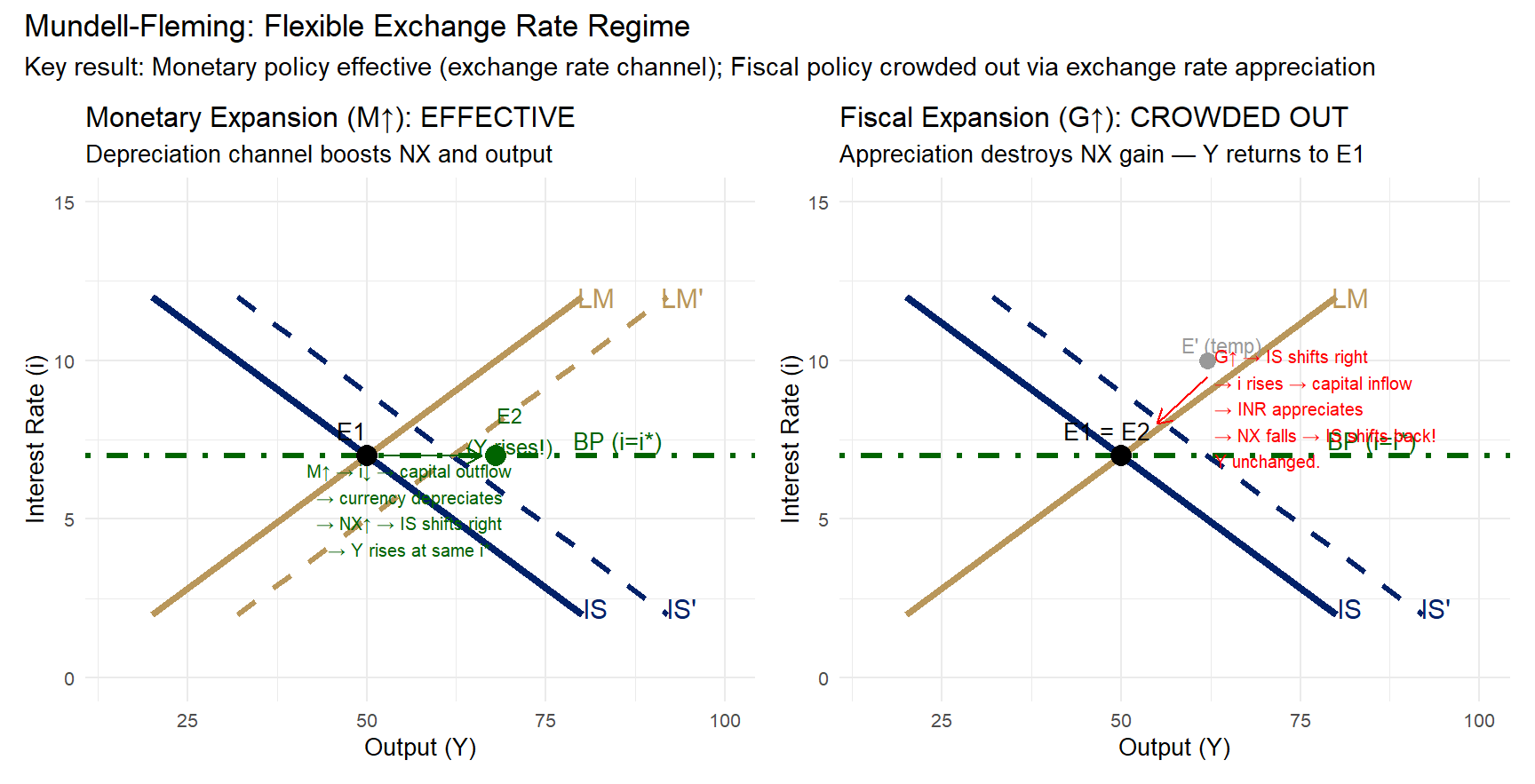
  labs(title="Monetary Expansion (M↑): EFFECTIVE",
       subtitle="Depreciation channel boosts NX and output",
       x="Output (Y)", y="Interest Rate (i)") +
  coord_cartesian(xlim=c(15,100), ylim=c(0,15)) +
  theme_minimal(base_size=10)

# Panel 2: Fiscal expansion under flexible (ineffective - crowded out)
p_fisc_flex <- ggplot() +
  geom_segment(aes(x=20, y=12, xend=80, yend=2), color="#012169", linewidth=1.5) +
  annotate("text", x=82, y=2.2, label="IS", size=4, color="#012169") +
  geom_segment(aes(x=32, y=12, xend=92, yend=2), color="#012169", linewidth=1.2, linetype="dashed") +
  annotate("text", x=94, y=2.2, label="IS'", size=4, color="#012169") +
  geom_segment(aes(x=20, y=12, xend=80, yend=2), color="#012169", linewidth=0.8, linetype="dotted") +
  geom_segment(aes(x=20, y=2, xend=80, yend=12), color="#B9975B", linewidth=1.5) +
  annotate("text", x=82, y=12, label="LM", size=4, color="#B9975B") +
  geom_hline(yintercept=7, linetype="dotdash", color="darkgreen", linewidth=1.2) +
  annotate("text", x=85, y=7.5, label="BP (i=i*)", size=3.5, color="darkgreen") +
  geom_point(aes(x=50, y=7), size=4, color="black") +
  geom_point(aes(x=62, y=10), size=3, color="grey60") +
  annotate("text", x=48, y=7.8, label="E1 = E2", size=3.5) +
  annotate("text", x=64, y=10.5, label="E' (temp)", size=3, color="grey60") +
  annotate("segment", x=62, y=9.5, xend=55, yend=8,
           arrow=arrow(length=unit(0.25,"cm")), color="red") +
  annotate("text", x=63, y=8.5,
           label="G↑ → IS shifts right\n→ i rises → capital inflow\n→ INR appreciates\n→ NX falls → IS shifts back!\nY unchanged.",
           size=2.7, color="red", hjust=0) +
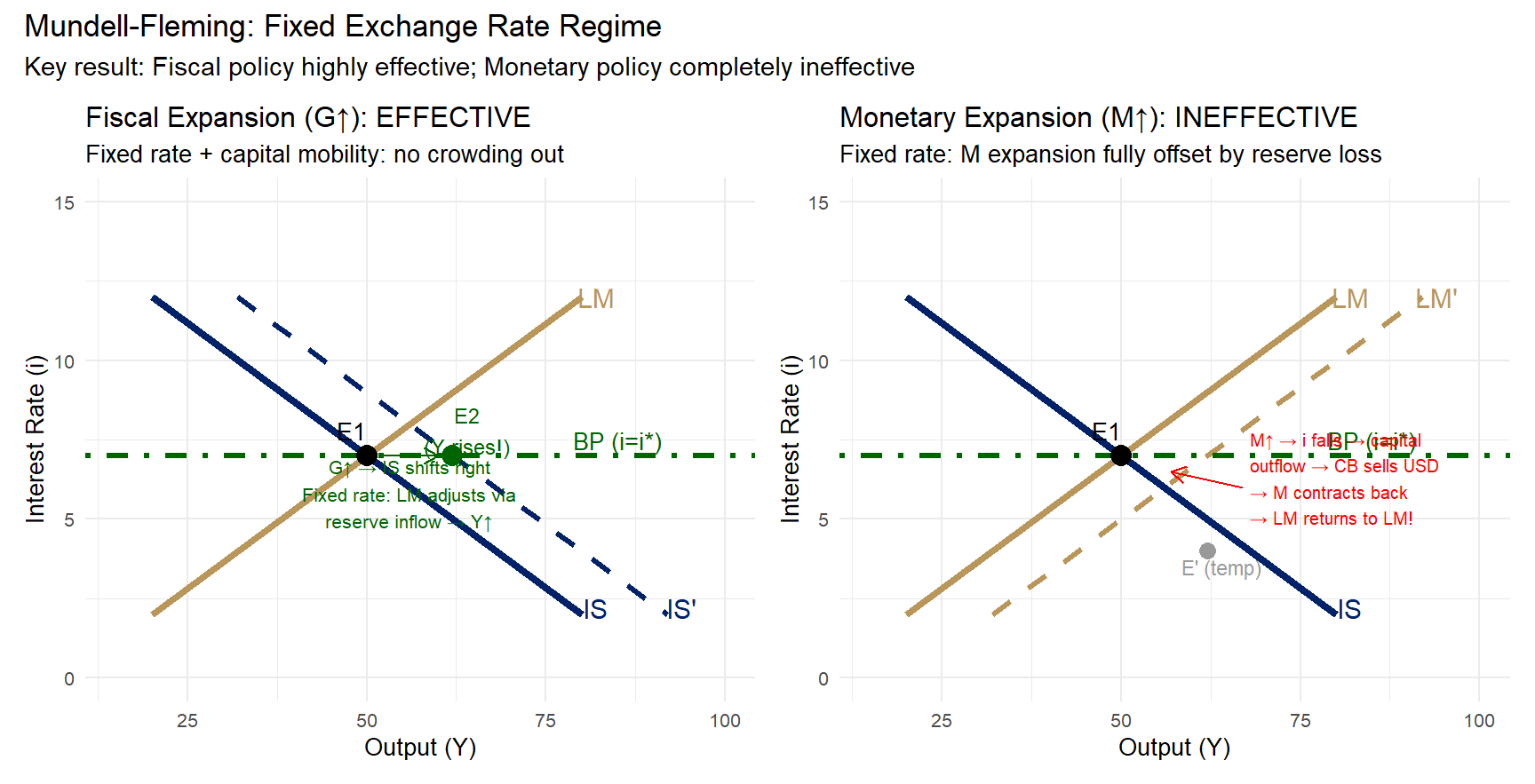
  labs(title="Fiscal Expansion (G↑): CROWDED OUT",
       subtitle="Appreciation destroys NX gain — Y returns to E1",
       x="Output (Y)", y="Interest Rate (i)") +
  coord_cartesian(xlim=c(15,100), ylim=c(0,15)) +
  theme_minimal(base_size=10)

p_mon_flex + p_fisc_flex +
  plot_annotation(
    title="Mundell-Fleming: Flexible Exchange Rate Regime",
    subtitle="Key result: Monetary policy effective (exchange rate channel); Fiscal policy crowded out via exchange rate appreciation"
  )

Figure 2

Mathematical mechanism — fiscal crowding out under flexible rate:

Under flexible \(e\): \(G\uparrow \Rightarrow Y\uparrow \Rightarrow M_d\uparrow \Rightarrow i\uparrow \Rightarrow\) capital inflow \(\Rightarrow\) INR appreciates \(\Rightarrow NX\downarrow \Rightarrow Y\) falls back

Agricultural implication under flexible rate: RBI rate cuts (monetary easing) boost agri exports via INR depreciation; fiscal spending on agriculture (e.g., PM-KISAN, PMFBY) may be partially crowded out by INR appreciation — reducing export competitiveness even as domestic support rises.

Mundell-Fleming: Policy Effectiveness Summary

Policy Fixed Rate Flexible Rate
Fiscal expansion (G↑) Effective — no crowding out, LM adjusts via reserves Ineffective — crowded out by exchange rate appreciation
Monetary expansion (M↑) Ineffective — fully offset by reserve loss Effective — works via exchange rate depreciation channel
Mechanism Reserve flows maintain fixed e Exchange rate adjusts to maintain BoP

Mundell’s insight (Nobel Prize 2000): The exchange rate regime determines which instruments of macroeconomic policy are effective. India’s managed float means both instruments have partial effectiveness — neither fully effective nor fully neutralised.

Agricultural policy implication: Under India’s managed float, RBI rate reductions (monetary easing) can boost INR exports through depreciation — but the effect is partial and conditional on RBI allowing the exchange rate to move. When RBI intervenes to prevent depreciation (to fight inflation), the monetary transmission via exchange rate is blocked.

India’s Forex Reserves: From Crisis to Abundance

Show R code
reserves <- data.frame(
  year = c(2000,2002,2004,2006,2008,2010,2012,2014,2016,2018,2020,2021,2022,2023,2024),
  reserves_b = c(38,67,141,199,310,297,296,322,366,405,580,642,532,620,645),
  months_import = c(5.1,9.8,14.2,13.4,9.8,9.5,6.8,8.1,10.5,9.2,15.8,14.1,9.4,11.5,11.0)
)

p1 <- ggplot(reserves, aes(x=year, y=reserves_b)) +
  geom_area(fill="#012169", alpha=0.25) +
  geom_line(color="#012169", linewidth=1.8) +
  geom_point(color="#012169", size=2.5) +
  annotate("text", x=2001, y=100, label="1991: $1.2B\n(only 2 weeks\nimport cover!)",
           size=2.8, color="red", hjust=0) +
  annotate("segment", x=2001, y=80, xend=2001, yend=45,
           arrow=arrow(length=unit(0.2,"cm")), color="red") +
  scale_x_continuous(breaks=seq(2000,2024,4)) +
  scale_y_continuous(labels=dollar_format(suffix="B", prefix="$")) +
  labs(title="India's Forex Reserves (USD Billion)",
       subtitle="From $38B (2000) to $645B (2024) — 17x increase",
       x=NULL, y="USD Billion") +
  theme_minimal(base_size=10)

p2 <- ggplot(reserves, aes(x=year, y=months_import)) +
  geom_line(color="#B9975B", linewidth=1.8) +
  geom_point(color="#B9975B", size=2.5) +
  geom_hline(yintercept=3, linetype="dashed", color="red", linewidth=1) +
  annotate("text", x=2016, y=3.6, label="Safety threshold: 3 months", size=3, color="red") +
  scale_x_continuous(breaks=seq(2000,2024,4)) +
  labs(title="Import Cover (Months of Imports)",
       subtitle="India currently has 11 months of import cover — well above the 3-month safety threshold",
       x=NULL, y="Months of Imports") +
  theme_minimal(base_size=10)

p1 / p2 + plot_annotation(title="India's Forex Reserves: From Crisis (1991) to Abundance (2024)")

Figure 3

\[\text{RBI's forex reserves} \approx \$645\text{B (FY2024)} \approx 11\text{ months of import cover}\]

Safety threshold = 3 months (Guidotti-Greenspan rule). India’s current buffer gives the RBI substantial firepower to defend the rupee in times of global turbulence. The $645B reserve stockpile is the direct product of 30 years of managed-float reserve accumulation — a deliberate policy choice to never repeat 1991.

RBI and India’s Managed Float

How RBI intervenes:

  • Depreciation prevention (INR falls too fast): RBI sells USD from reserves, absorbing rupees → reduces money supply → supports INR
  • Appreciation prevention (INR rises too fast): RBI buys USD, injecting rupees → increases money supply → weakens INR

Sterilization mechanism:

\[\Delta \text{Reserves} + \Delta \text{Domestic Credit} = \Delta M\]

When RBI buys USD → \(\Delta M\) (base money rises) → RBI sells G-secs (government securities) to sterilize — absorbing ₹ and keeping money supply neutral.

Two-way intervention (managed float):

  • Sell USD when INR weakens sharply (e.g., 2022)
  • Buy USD when INR strengthens too fast (e.g., 2021)
  • Sterilisation uses liquidity operations (OMOs, reverse repo, etc.)

RBI’s two-way intervention evidence: - FY2021: Net purchases ~$67B (preventing appreciation during COVID capital inflows) - FY2022–23: Net sales ~$100B (preventing excessive depreciation) - IMF and US Treasury classification: India is NOT a currency manipulator — two-way intervention distinguishes managed float from competitive devaluation.

The Forward Exchange Market (idea)

  • A forward locks in an exchange rate today for a future date

\[\text{Forward premium} = \frac{F - E}{E} \times \frac{12}{n} \times 100\%\]

Example (3-month): \(E=₹83.5/\$\), \(F=₹84.2/\$\) → premium ≈ 3.35% p.a.

Who uses forwards (agri context)

  • Large exporters: lock in INR realisation on USD receipts
  • Large importers (edible oils, fertiliser): lock in INR cost of USD payments
  • Small farmers/FPOs have limited direct access (scale + documentation)

Hedging with a forward (diagram)

Show R code
e_future <- seq(78, 92, by=0.25)
unhedged <- e_future * 10
hedged_rate <- 84.2
hedged <- rep(hedged_rate * 10, length(e_future))

df_hedge <- data.frame(
  e_future = e_future,
  unhedged = unhedged,
  hedged = hedged
)

df_hedge_below <- df_hedge[df_hedge$e_future <= hedged_rate, ]
df_hedge_above <- df_hedge[df_hedge$e_future >= hedged_rate, ]

ggplot(df_hedge, aes(x=e_future)) +
  geom_ribbon(data=df_hedge_below,
              aes(x=e_future, ymin=unhedged, ymax=hedged),
              fill="darkgreen", alpha=0.2) +
  geom_ribbon(data=df_hedge_above,
              aes(x=e_future, ymin=hedged, ymax=unhedged),
              fill="#cc0000", alpha=0.15) +
  geom_line(aes(y=unhedged, color="Unhedged"), linewidth=1.4) +
  geom_line(aes(y=hedged, color="Hedged (forward)"), linewidth=1.4, linetype="dashed") +
  geom_vline(xintercept=hedged_rate, linetype="dotted", color="grey40") +
  scale_color_manual(values=c("Unhedged"="#012169","Hedged (forward)"="#B9975B")) +
  labs(title="Rice exporter: hedging a $10M receivable",
       subtitle="Forward at ₹84.2/$ fixes INR receipts; hedge trades off upside for certainty",
       x="Future spot rate (₹ per $)", y="INR received (crores)", color=NULL) +
  theme_minimal(base_size=11) +
  theme(legend.position="bottom")

Figure 4

Access gap: OTC vs futures

  • OTC forwards typically require large minimum sizes
  • Exchange-traded currency futures have smaller lot sizes but require margin + daily mark-to-market

In practice, hedging is much easier for large firms than for small farmers and FPOs.

Exchange Rate Pass-Through

Definition: The pass-through coefficient \(\psi\) measures how much of an exchange rate change is reflected in domestic import prices.

\[\psi = \frac{\% \Delta P^{import}}{\% \Delta e}\]

  • If \(\psi = 1\) (complete pass-through): 10% INR depreciation → 10% rise in import prices (exporters maintain foreign-currency price)
  • If \(\psi < 1\) (incomplete): foreign exporters absorb some of the change in their margins (especially for branded/differentiated goods)

General formula:

\[\Delta P^{import} = \psi \cdot \Delta e + \text{world price change}\]

India estimates:

  • Edible oil: \(\psi \approx 0.7\)\(0.85\) (high — palm oil is homogeneous, world price sets import price)
  • Manufactured imports: \(\psi \approx 0.4\)\(0.6\) (lower — brand and quality differentiation)
  • Petroleum products: \(\psi \approx 0.9\) (nearly complete — global commodity)

India’s edible-oil channel (rule of thumb):

  • INR depreciation raises the ₹ price of imported edible oils
  • ₹10/$ depreciation (e.g., ₹75 → ₹85) → roughly ₹8–9/litre higher retail price (high pass-through)
  • With ~20 Mt consumption (~1.4 bn litres), ₹9/litre ≈ ₹12,600 crore/year added consumer cost

Exchange rate policy and food inflation policy are tightly linked.

INR Depreciation and Agricultural Exports

Show R code
agri_inr <- data.frame(
  year = 2010:2024,
  inr_usd = c(45.7,46.7,53.4,60.1,61.0,65.5,67.1,65.1,69.9,70.4,
              74.1,73.9,76.2,82.6,83.5),
  agri_exports = c(18,26,36,39,42,43,34,33,38,40,41,50,53,54,53)
)

ggplot(agri_inr, aes(x=inr_usd, y=agri_exports)) +
  geom_point(color="#012169", size=3.2) +
  geom_smooth(method="lm", se=TRUE, color="#B9975B", fill="#B9975B", alpha=0.2) +
  geom_text(aes(label=year), nudge_y=0.8, size=2.6, color="grey40") +
  labs(title="INR/USD vs agri exports (FY2010–FY2024)",
       subtitle="Weaker INR often coincides with higher agri exports (USD)",
       x="INR per USD (year average)", y="Agri exports (USD bn)") +
  theme_minimal(base_size=11)

Figure 5

What to take from the plot

  • Often: weaker INR ↔︎ higher exports (USD), especially for price-sensitive commodities
  • But global prices + demand also move exports (commodity cycle)
  • Causality can run both ways (trade balance shocks can also move INR)
  • Example: 2013–14 INR fell ~15% and rice exports surged

Competitiveness arithmetic (rule of thumb)

  • ₹75/$ → ₹83/$ increases INR per $ by about 10.7%
  • If USD export price is unchanged, exporter gets ~10.7% more INR per $
  • Symmetrically, importers face a cost shock in rupees

Exchange rate movements act like an implicit export subsidy / import tax (without a budget line).

India’s edible oil vulnerability (headline)

  • Imports ≈ 14–16 Mt per year (large import dependence)
  • Major sources: Indonesia/Malaysia (palm), Argentina/Brazil (soy), Black Sea (sunflower)
  • Exchange rate movements feed into domestic cooking-oil inflation

Exchange rate arithmetic (simple)

  • If world palm oil price is fixed in USD, a weaker INR raises the ₹/tonne cost
  • Example: moving from ₹75/$ → ₹85/$ raises rupee cost by ~13% (holding USD price constant)

Policy levers and the “duty floor” problem

  • Duty cuts can cushion price spikes, but 0% is the floor
  • Once duties are cut, INR depreciation still passes through to prices
  • Edible oils therefore link exchange rates to food inflation

Edible oils are the cleanest channel where exchange rate policy becomes food policy.

Managing Currency Risk in Agricultural Trade

Agri Exporters (risk: INR appreciates, reducing INR revenue)

  • Forward sales: lock in ₹/$ today for future USD receipt — eliminate downside but sacrifice upside
  • Export credit in USD (ECB): borrow in USD, repay with export proceeds — no currency conversion needed
  • Put options on USD: right to sell USD at floor price — limits downside while retaining upside

Agri Importers (risk: INR depreciates, raising ₹ cost)

  • Forward purchases: lock in ₹/$ for future USD payment — certainty on import cost
  • Call options on USD: right to buy USD at ceiling price — caps cost if INR weakens

BoP and the Current Account (CAD): the agri connection

  • Identity: CA + KA + FA = 0
  • India’s CAD is usually ~1.5–2.5% of GDP
  • Big CAD pressure often comes from oil/fertiliser (USD-priced) imports

CAD drivers (FY2024, rough magnitudes)

  • Merchandise trade balance: about −$300B
  • Services balance: about +$150B
  • Remittances: about +$100B
  • Primary income: about −$30B

Order-of-magnitude: CAD ≈ −$80B in FY2024.

Agriculture as an offset (and feedback)

  • Agri trade is often a +$20–25B surplus (FY2024 ≈ +$25B)
  • Major items: rice, marine products, spices, sugar, cotton
  • Feedback logic: weaker INR can lift agri exports → improves CA → reduces pressure on RBI reserves

Key Takeaways: Lecture 12

Five core concepts from Lecture 12:

  1. Exchange rate regimes: Free float (USA), managed float (India), fixed (Gulf). India’s managed float (post-1993) preserves partial monetary independence at the cost of active reserve management ($645B stockpile).

  2. Impossible Trinity: Cannot have all three of fixed rate + free capital + monetary independence. India chooses partial versions of all three — a pragmatic compromise that gives flexibility without full commitment to any extreme.

  3. Mundell-Fleming model:

    • Fixed rate: Fiscal policy effective (\(G\uparrow \Rightarrow Y\uparrow\)); Monetary policy ineffective (\(M\uparrow\) offset by reserve loss)
    • Flexible rate: Monetary policy effective (\(M\uparrow \Rightarrow e\uparrow \Rightarrow NX\uparrow \Rightarrow Y\uparrow\)); Fiscal crowded out by appreciation
  4. Hedging: Forward contracts lock in exchange rate for future transactions; essential for large agri exporters/importers. CIP ensures forward premium = interest differential. Small farmers cannot access these instruments — a key equity gap.

  5. Agriculture–exchange rate nexus: Depreciation helps rice/cotton/spice exporters (direct competitiveness); hurts edible oil/fertiliser importers (cost inflation); RBI’s managed float attempts to balance these competing interests through two-way intervention.

Exchange Rates as Agricultural Trade Policy

Exchange rate policy IS trade policy in disguise:

A country that keeps its currency undervalued effectively subsidises all its exports and taxes all its imports — without any WTO-notifiable expenditure.

China’s managed undervaluation (2000s):

  • RMB/USD held artificially low through massive reserve accumulation ($3T+)
  • Made Chinese agri exports (garlic, processed food, aquaculture) highly competitive globally
  • Undercut Indian agri exporters in third markets — without any explicit subsidy

Brazil’s floating BRL — competitive depreciation by market:

  • BRL/USD fell ~50% in 2015–16 (from BRL 2.5 → BRL 4.0/$)
  • Made Brazilian soy, beef, chicken dramatically cheaper in USD terms
  • Directly hurt Indian soy farmers and agri exporters in overlapping markets
  • India had no “WTO case” — Brazil’s depreciation was market-driven, not policy-directed

India’s REER concern:

  • If India’s Real Effective Exchange Rate (REER) rises (INR appreciates in real terms relative to trading partners), agri exports face headwind regardless of domestic MSP levels
  • REER = nominal exchange rate × (domestic price level / foreign price level) — captures competitiveness
  • India’s REER has trended upward since 2014 (relatively higher inflation than trading partners + nominal rupee stability)

WTO and exchange rates — a critical gap:

WTO disciplines agricultural subsidies (AoA Agreement) but does NOT discipline exchange rate policy. Countries can gain large competitive advantages in agricultural trade through currency policy — without violating WTO commitments. This is a major structural asymmetry in international trade rules: a $1B MSP subsidy is notifiable and challengeable; a $50B reserve accumulation that undervalues the currency is not. The IMF (not WTO) has jurisdiction on exchange rate manipulation — but enforcement is weak.

Next Lecture: Balance of Payments Analysis

Lecture 13 (July 18, 2026): Balance of Payments: Structure, Adjustment, and Agricultural Trade

We will cover:

  • Current account, capital account, financial account structure
  • BoP adjustment mechanisms: automatic vs policy-driven
  • Marshall-Lerner condition: when does depreciation improve the trade balance?
  • J-curve effect: short-run vs long-run response to depreciation
  • India’s current account deficit: causes and sustainability

Appendix

Additional Resources

Further reading

  • Salvatore, International Economics (relevant chapters)
  • Appleyard & Field, International Economics (relevant chapters)

Key data sources

  • DGCI&S: merchandise trade
  • RBI: exchange rates + BoP
  • APEDA: agricultural export statistics
  • WTO: tariff + trade databases