Lecture 11: Foreign Exchange — Rates and Determination

Econ 2203 | International Trade and Policy in Agriculture

Nithin M

Department of Development Economics

2026-07-04

Foreign Exchange: Rates and Determination

How the rupee’s price against the dollar shapes India’s agricultural exports, food prices, and farmer incomes — and what economic theory tells us about why exchange rates move.

What is an Exchange Rate?

The nominal exchange rate is the price of one currency in terms of another.

\[e = \text{units of domestic currency per unit of foreign currency}\]

\[e_{INR/USD} = 83.5 \Rightarrow \text{1 USD costs }₹83.5\]

• Direct quote (India convention): ₹ per USD — how many rupees to buy 1 dollar
• Indirect quote: USD per ₹ — how many dollars 1 rupee buys (= 1/83.5 = $0.012)

India 2024: The RBI reference rate hovered near ₹83–84/USD throughout 2024. A software exporter invoicing $1M receives ₹83.5 crore at spot. A food importer buying $1M of edible oil pays ₹83.5 crore. The same rate creates winners and losers simultaneously.

Spot vs Forward Rates

Feature	Spot Rate	Forward Rate
Settlement	Immediate (T+2)	Agreed today, settled at future date
Certainty	Current market price	Locked-in price for future delivery
India example	₹83.5/$	3-month forward: ₹84.2/$
Use	Immediate trade settlement	Hedging future currency exposure

Forward premium calculation:

\[\text{Forward Premium (p.a.)} = \frac{F - E}{E} \times \frac{12}{n} \times 100 = \frac{84.2 - 83.5}{83.5} \times 4 \times 100 = 3.35\%\]

Why forward rates matter for agri exporters: An Indian basmati exporter signing a 3-month USD contract today faces uncertainty — if INR appreciates by delivery, they receive fewer rupees. By selling USD forward at ₹84.2/$, they lock in their revenue. The forward premium (3.35%) reflects market expectations of INR depreciation.

Nominal vs Real Exchange Rate

The nominal rate tells us the currency price. The real rate tells us purchasing power competitiveness.

\[q = e \cdot \frac{P^*}{P}\]

where \(q\) = real exchange rate, \(e\) = nominal rate (₹/$), \(P^*\) = US price level, \(P\) = India price level.

Numerical example — Basmati Rice:

• India price: ₹5,010/quintal; US equivalent: $60/quintal; \(e\) = ₹83.5/$
• \(q = 83.5 \times (60/5{,}010) = 83.5 \times 0.01197 = 0.999 \approx 1\)
• If India inflation pushes price to ₹5,600 with same nominal \(e\): \(q = 83.5 \times (60/5{,}600) = 0.894\) → INR real appreciation → Indian rice less competitive even though nominal rate unchanged

Why the real rate is what matters for trade competitiveness: India’s nominal exchange rate may be stable, but if domestic inflation outpaces foreign inflation, Indian goods become relatively expensive. Only a real depreciation — either a nominal depreciation or lower relative inflation — genuinely improves export competitiveness.

Real Effective Exchange Rate (REER): Trade-weighted average across all trading partners:

\[\text{REER} = \prod_i \left(e_i \cdot \frac{P_i^*}{P}\right)^{w_i}\]

Appreciation vs Depreciation

The key rule: If \(e\) rises (more ₹ per $) → INR depreciates. If \(e\) falls → INR appreciates.

INR Depreciation (e ↑, e.g. ₹75→₹85)

• ✅ Cotton exporters: same USD price = more ₹ revenue
• ✅ Rice exporters (world’s No.1): Indian rice cheaper for foreign buyers
• ✅ Spice/marine exporters: competitive advantage
• ❌ Edible oil importers: same $ price = more ₹ cost → higher cooking oil prices

INR Appreciation (e ↓, e.g. ₹85→₹75)

• ✅ Edible oil importers: cheaper palm, soybean, sunflower oil
• ✅ Pulses importers: cheaper lentils from Canada/Australia
• ✅ Fertiliser importers: urea, DAP cheaper in ₹
• ❌ Rice exporters: Indian rice more expensive globally → volume loss

Additional depreciation effects:

• ❌ Fertiliser importers: input costs rise → squeezes farmer margins
• ❌ Food inflation: imported food basket becomes expensive

Additional appreciation effects:

• ✅ Consumers: lower food inflation
• ❌ Cotton exporters: margins squeezed
• ❌ Spice/marine sector: competitiveness falls

Demand for Foreign Exchange

Who demands USD (buys USD, sells ₹)?

• 🛢️ Importers (crude oil, edible oil, electronics, machinery)
• 💸 Capital outflows (Indian firms investing abroad, FPI selling)
• ✈️ Tourism abroad (Indians travelling overseas)
• 🏦 Debt repayments (external commercial borrowings in USD)
• 📉 FPI outflows (foreign portfolio investors exiting India)

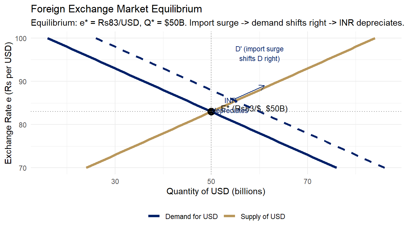
Demand function: As \(e\) rises (INR depreciates), imports become expensive → quantity of USD demanded falls.

\[Q_D = 216 - 2e\]

where \(e\) is ₹ per USD and \(Q\) is billions of USD. Downward-sloping demand curve.

Agricultural angle: India’s edible oil imports (~$14B/year) are the largest agricultural component of USD demand — palm oil from Indonesia/Malaysia, soybean oil from Argentina/Brazil, sunflower oil from Ukraine. A weaker rupee makes every litre more expensive.

Supply of Foreign Exchange

Who supplies USD (sells USD, buys ₹)?

• 📦 Exporters (IT services, rice, spices, cotton, pharmaceuticals) — earn USD, convert to ₹
• 🏭 FDI inflows (foreign firms investing in India)
• 📈 FPI inflows (foreign portfolio investors buying Indian stocks/bonds)
• 💰 Remittances — largest single source at ~$100B/year (> FDI of $71B in FY2023)
• 🏦 External borrowings (ECBs, NRI deposits)

Supply function: As \(e\) rises (INR weakens), Indian exports are cheaper globally → more exported → more USD earned and supplied.

\[Q_S = -116 + 2e\]

Upward-sloping supply curve. When \(e\) is high, each dollar of export revenue translates to more rupees — incentivising more exports.

Agricultural note: Rice ($10B+), spices ($4B+), cotton ($2B+), marine products ($8B+) are key agri supply sources of USD. A weak rupee boosts these exports.

Foreign Exchange Market Equilibrium

e_seq <- seq(70, 100, by=0.5)
Q_d2 <- 216 - 2*e_seq
Q_s2 <- -116 + 2*e_seq

df_forex <- data.frame(
  e = e_seq,
  Q_d = pmax(0, Q_d2),
  Q_s = pmax(0, Q_s2)
)

df_d_shift <- data.frame(
  Q = pmax(0, 226 - 2*e_seq),
  e = e_seq
)

ggplot(df_forex) +
  geom_line(aes(x=Q_d, y=e, color="Demand for USD"), linewidth=1.5) +
  geom_line(aes(x=Q_s, y=e, color="Supply of USD"), linewidth=1.5) +
  geom_point(aes(x=50, y=83), size=4, color="black") +
  annotate("text", x=52, y=83.8, label="E* (Rs83/$, $50B)", size=3.5, hjust=0) +
  geom_hline(yintercept=83, linetype="dotted", color="grey50") +
  geom_vline(xintercept=50, linetype="dotted", color="grey50") +
  geom_line(data=df_d_shift, aes(x=Q, y=e), color="#012169", linetype="dashed", linewidth=1.1) +
  annotate("text", x=60, y=96.5, label="D' (import surge\nshifts D right)", size=3, color="#012169") +
  annotate("segment", x=55, y=86, xend=61, yend=89,
           arrow=arrow(length=unit(0.25,"cm")), color="#012169") +
  annotate("text", x=54, y=84.5, label="INR\ndepreciates", size=3, color="#012169") +
  scale_color_manual(values=c("Demand for USD"="#012169", "Supply of USD"="#B9975B")) +
  labs(title="Foreign Exchange Market Equilibrium",
       subtitle="Equilibrium: e* = Rs83/USD, Q* = $50B. Import surge -> demand shifts right -> INR depreciates.",
       x="Quantity of USD (billions)", y="Exchange Rate e (Rs per USD)",
       color=NULL) +
  theme(legend.position="bottom")

Figure 1: Foreign Exchange Market: Equilibrium Exchange Rate Determination Source: Author’s illustration.

Solving for equilibrium: Set \(Q_D = Q_S\):

\[216 - 2e = -116 + 2e \Rightarrow 332 = 4e \Rightarrow e^* = 83, \quad Q^* = 50\]

Factors Shifting Demand and Supply

Factor	Shift	Effect on e (₹/$)	INR
India inflation ↑	D shifts right	e ↑	Depreciates
India growth ↑ → imports ↑	D shifts right	e ↑	Depreciates
FDI/FPI outflows ↑	D shifts right	e ↑	Depreciates
Oil prices ↑	D shifts right	e ↑	Depreciates
Export earnings ↑	S shifts right	e ↓	Appreciates
FDI/FPI inflows ↑	S shifts right	e ↓	Appreciates
Remittances ↑	S shifts right	e ↓	Appreciates
RBI raises rates	S shifts right (capital inflows)	e ↓	Appreciates

Reading the table: Every factor works through either the current account (trade in goods/services) or the capital/financial account (investment flows). The 2013 “Taper Tantrum” combined FPI outflows (D↑) with reduced remittances to trigger the sharpest post-2008 INR depreciation.

India INR/USD Trend (2008–2024)

inr_events <- data.frame(
  year = c(2008,2009,2010,2011,2012,2013,2014,2015,2016,2017,
           2018,2019,2020,2021,2022,2023,2024),
  rate = c(43.5,48.4,45.7,46.7,53.4,60.1,61.0,65.5,67.1,65.1,
           69.9,70.4,74.1,73.9,79.8,82.6,83.5)
)

events <- data.frame(
  year  = c(2008,  2013,       2016,                2018,               2022),
  rate  = c(43.5,  60.1,       67.1,                70.4,               79.8),
  label = c("GFC\n2008","Taper\nTantrum","Demonetisation\n+Trump","Oil crisis\n+capital flight","Ukraine war\n+USD surge")
)

ggplot(inr_events, aes(x=year, y=rate)) +
  geom_line(color="#012169", linewidth=1.8) +
  geom_point(color="#012169", size=2) +
  geom_point(data=events, aes(x=year, y=rate), color="#B9975B", size=4) +
  geom_text(data=events, aes(x=year, y=rate+2.5, label=label),
            size=2.8, color="#B9975B", vjust=0, lineheight=0.9) +
  scale_x_continuous(breaks=seq(2008,2024,2)) +
  labs(title="India's INR/USD Exchange Rate (2008–2024)",
       subtitle="INR depreciated from Rs43 to Rs83/USD over 16 years — inflation differentials + global shocks",
       x=NULL, y="Rs per USD (higher = weaker INR)") +
  theme_minimal(base_size=11)

Figure 2: INR/USD Exchange Rate: Key Depreciation Episodes (2008–2024) Source: RBI, Database on Indian Economy (DBIE).

• 2008 GFC: Global risk-off → capital flight from EMs. Rice/agri export demand fell; edible oil imports also dropped.
• 2013 Taper Tantrum: Fed signalled rate hike → FPI outflows. Cotton, rice exporters saw ₹ revenue spike but volatile.
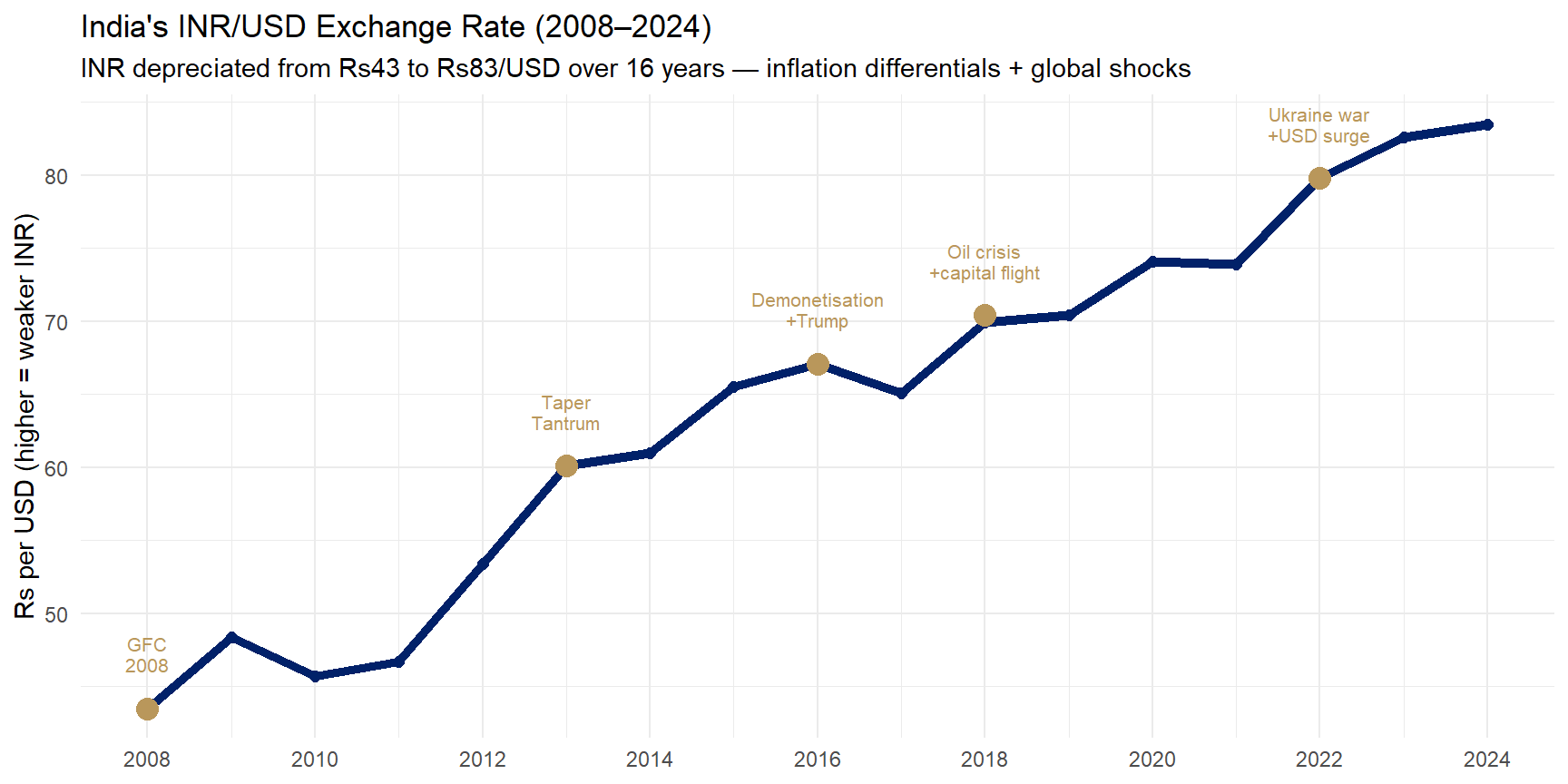
• 2018: Iran sanctions + crude oil surge. India’s $150B crude import bill inflated → INR hit ₹75.
• 2022 Ukraine: Sunflower oil import disruption + USD surge → edible oil crisis in India.

Purchasing Power Parity: Absolute PPP

Foundation — Law of One Price: In competitive markets with free trade, identical goods sell at the same price internationally (once converted at the exchange rate).

Absolute PPP: If a representative basket costs ₹4,175 in India and $50 in the USA:

\[e_{PPP} = \frac{P_{India}}{P_{USA}} = \frac{4175}{50} = ₹83.5 \text{ per USD}\]

Absolute PPP says: the exchange rate should equal the ratio of price levels. If the actual rate differs from PPP, there is a real misalignment.

Big Mac Index 2024 — Reality Check:

Item	India	USA
Big Mac price	₹259	$5.69
Implied PPP	₹259/\(5.69 = **₹45.5/\)**	—
Actual rate	₹83.5/$	—
Verdict	INR undervalued by ~45% vs PPP	—

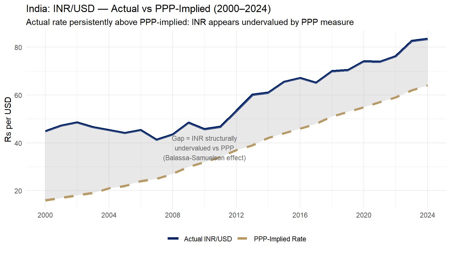
This does not mean INR is “wrong” — it reflects real structural differences (Balassa-Samuelson effect, see Slide 13).

Relative PPP

Relative PPP: Exchange rates change in proportion to inflation differentials.

\[\% \Delta e \approx \pi_{India} - \pi_{USA}\]

Numerical example:

If India’s inflation \(\pi_{India} = 5\%\) and USA’s \(\pi_{USA} = 2\%\):

\[\% \Delta e = 5\% - 2\% = +3\% \Rightarrow \text{INR depreciates 3\% per year}\]

Long-run empirical test for India:

• ₹45/USD (2000) → ₹83.5/USD (2024): 85.6% depreciation over 24 years → ~3.5% per year
• India avg CPI inflation (2000–2024): ~5.5%; US avg: ~2.2% → differential ≈ 3.3%
• ✓ Broadly consistent with Relative PPP!

Agricultural implication: Relative PPP predicts that India’s ~3–4% annual INR depreciation roughly offsets the ~3% domestic cost inflation facing Indian farmers. This means Indian agri exports maintain their global price competitiveness in the long run — inflation at home is offset by depreciation in the exchange rate. Short-run deviations, however, create real competitive swings.

India: PPP-Implied vs Actual Rate

inr_data <- data.frame(
  year = 2000:2024,
  actual = c(44.9,47.2,48.6,46.6,45.3,44.1,45.3,41.3,43.5,48.4,
             45.7,46.7,53.4,60.1,61.0,65.5,67.1,65.1,69.9,70.4,
             74.1,73.9,76.2,82.6,83.5),
  ppp_implied = c(16,17,18,19,21,22,24,25,27,30,
                  32,34,37,39,42,44,46,48,51,53,
                  55,57,59,62,64)
)

ggplot(inr_data, aes(x=year)) +
  geom_line(aes(y=actual, color="Actual INR/USD"), linewidth=1.5) +
  geom_line(aes(y=ppp_implied, color="PPP-Implied Rate"), linewidth=1.5, linetype="dashed") +
  geom_ribbon(aes(ymin=ppp_implied, ymax=actual), fill="grey70", alpha=0.3) +
  annotate("text", x=2010, y=38, label="Gap = INR structurally\nundervalued vs PPP\n(Balassa-Samuelson effect)",
           size=3, color="grey40") +
  scale_color_manual(values=c("Actual INR/USD"="#012169","PPP-Implied Rate"="#B9975B")) +
  scale_x_continuous(breaks=seq(2000,2024,4)) +
  labs(title="India: INR/USD — Actual vs PPP-Implied (2000–2024)",
       subtitle="Actual rate persistently above PPP-implied: INR appears undervalued by PPP measure",
       x=NULL, y="Rs per USD", color=NULL) +
  theme_minimal(base_size=11) +
  theme(legend.position="bottom")

Figure 3: India: Actual Exchange Rate vs PPP-Implied Rate (INR/USD, 2000–2024) Source: RBI; World Bank, International Comparison Program (ICP).

Balassa-Samuelson Effect: Fast-growing economies (like India) have high productivity growth in tradables (IT, manufacturing) but not in non-tradables (haircuts, local food). This raises wages overall, making non-tradables expensive. PPP calculations using full CPI baskets therefore understate the “true” exchange rate for a developing economy — the gap between actual and PPP-implied is structurally expected, not a sign of manipulation.

Limitations of PPP

PPP is a powerful long-run benchmark but has important practical limitations:

1. Non-tradable goods — haircuts, education, land, local restaurants don’t arbitrage across borders. Their prices differ permanently.
2. Quality differences — a “Big Mac” in Tokyo ≠ a Big Mac in Delhi in quality perception.
3. Trade barriers — tariffs, quotas, and transport costs prevent price equalisation even for tradables.
4. Balassa-Samuelson effect — richer/faster-growing countries systematically have currencies above PPP because productivity gains in tradables spill over to raise wages in non-tradables.
5. Short-run irrelevance — capital flows, sentiment, and central bank intervention dominate short-run exchange rates. PPP explains long-run trends, not day-to-day movements.

Agricultural implication: Agricultural commodities — rice, wheat, cotton, edible oils, spices — ARE tradable goods. PPP-based analysis is therefore more applicable to food prices than to services prices. When the IMF/World Bank assess food affordability across countries, they use PPP-adjusted incomes. India’s apparent INR undervaluation by PPP helps explain why Indian agricultural exports are consistently price-competitive globally.

Interest Rate Parity: Uncovered IRP

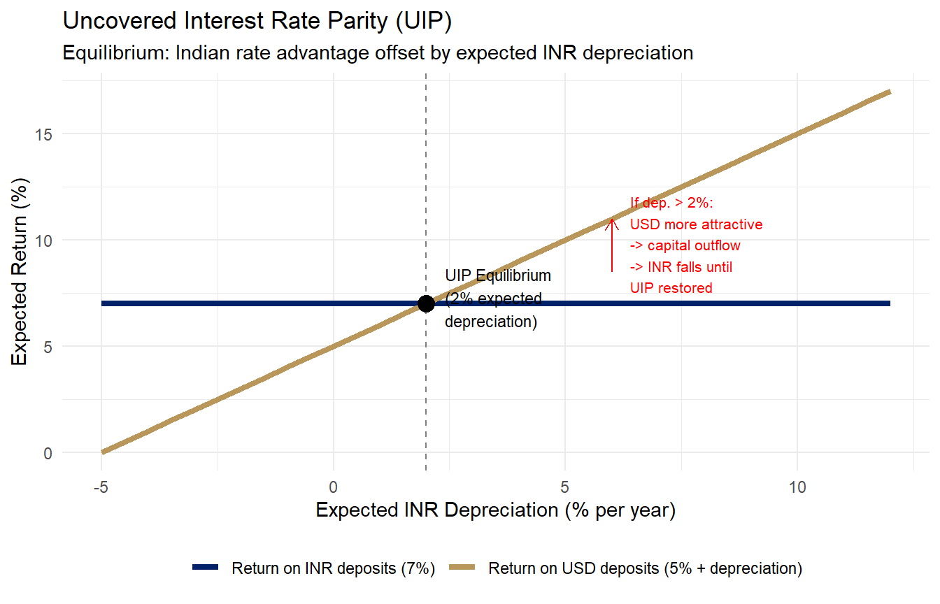
Setup: An Indian investor has ₹1 crore to invest for 1 year. Two options:

1. INR bond earning \(i_{India} = 7\%\) → get ₹1.07 crore in 1 year
2. USD bond earning \(i_{USA} = 5\%\), but must convert ₹ to $ now and $ back to ₹ later

Uncovered Interest Rate Parity (UIP): In equilibrium, expected returns must be equal:

\[i_{India} = i_{USA} + \frac{E^e - E}{E}\]

where \(E^e\) = expected future exchange rate (uncertain — hence “uncovered”).

Rearranged:

\[\frac{E^e - E}{E} = i_{India} - i_{USA} = 7\% - 5\% = 2\%\]

→ Market expects INR to depreciate 2% per year to equalise returns.

Interpretation: India’s higher interest rates do NOT simply attract unlimited capital inflows — because investors price in the expected currency depreciation. The interest rate advantage is exactly offset (in equilibrium) by the expected loss from holding a depreciating currency. This is why India cannot run 8% rates indefinitely without currency pressure.

UIP Diagram

depreciation_pct <- seq(-5, 12, by=0.5)
i_usd <- 5
return_usd <- i_usd + depreciation_pct

df_irp <- data.frame(
  dep = depreciation_pct,
  return_inr = 7,
  return_usd = return_usd
)

ggplot(df_irp, aes(x=dep)) +
  geom_line(aes(y=return_inr, color="Return on INR deposits (7%)"), linewidth=1.5) +
  geom_line(aes(y=return_usd, color="Return on USD deposits (5% + depreciation)"), linewidth=1.5) +
  geom_vline(xintercept=2, linetype="dashed", color="grey50") +
  geom_point(aes(x=2, y=7), size=4, color="black") +
  annotate("text", x=2.4, y=7.3, label="UIP Equilibrium\n(2% expected\ndepreciation)", size=3, hjust=0) +
  annotate("segment", x=6, y=8.5, xend=6, yend=11.0,
           arrow=arrow(length=unit(0.25,"cm")), color="red") +
  annotate("text", x=6.4, y=9.8, label="If dep. > 2%:\nUSD more attractive\n-> capital outflow\n-> INR falls until\nUIP restored",
           size=2.8, color="red", hjust=0) +
  scale_color_manual(values=c("Return on INR deposits (7%)"="#012169",
                               "Return on USD deposits (5% + depreciation)"="#B9975B")) +
  labs(title="Uncovered Interest Rate Parity (UIP)",
       subtitle="Equilibrium: Indian rate advantage offset by expected INR depreciation",
       x="Expected INR Depreciation (% per year)", y="Expected Return (%)",
       color=NULL) +
  theme_minimal(base_size=11) +
  theme(legend.position="bottom")

Figure 4: Uncovered Interest Rate Parity: Expected Return Equalization Source: Author’s illustration.

Covered vs Uncovered IRP

Covered Interest Rate Parity (CIP): Uses the forward exchange rate — no uncertainty.

\[i_{India} = i_{USA} + \frac{F - E}{E}\]

where \(F\) = forward exchange rate (agreed today, settled at future date — no currency risk).

Uncovered Interest Rate Parity (UIP): Uses the expected future spot rate — uncertain.

\[i_{India} = i_{USA} + \frac{E^e - E}{E}\]

Empirical verdict:

• CIP holds almost perfectly in practice — arbitrage desks enforce it millisecond-to-millisecond.
• UIP weaker empirically — exchange rate risk premium and investor irrationality cause deviations.

Numerical CIP check (India, 2024):

• Spot \(E\) = ₹83.5/$; 3-month forward \(F\) = ₹84.2/$
• Forward premium = \((84.2-83.5)/83.5 \times 4 \times 100 = 3.35\%\) p.a.
• Interest differential: \(i_{India}=6.5\%\), \(i_{USA}=5.3\%\) → \(\Delta i = 1.2\%\)
• Gap (3.35% vs 1.2%) is explained by country risk premium on Indian sovereign debt.

Agri exporter hedging via CIP: A rice exporter expecting \(5M in 6 months sells USD forward at ₹84.2/\). CIP guarantees the forward rate is fairly priced relative to the interest differential — no “free money” from hedging, but the exporter eliminates revenue uncertainty. The forward premium (3.35%) is the cost of certainty.

RBI Intervention in the Forex Market

How RBI intervenes:

• Preventing excessive depreciation: RBI sells USD from reserves → increases USD supply in market → reduces e (strengthens INR)
• Preventing excessive appreciation: RBI buys USD → reduces USD supply → increases e (weakens INR)

Sterilisation mechanism:

When RBI buys USD (injects ₹ into economy): 1. Buy USD → ₹ liquidity increases (inflationary) 2. Simultaneously sell government securities (G-secs) → absorbs ₹ back 3. Net effect: money supply neutral, but forex reserves increase

India’s forex reserve trajectory:

Year	Reserves	Import cover
1991	$1.2B	2 weeks (crisis)
2004	$113B	~12 months
2014	$304B	~8 months
2024	~$645B	~11 months

Sterilisation and agriculture:

When RBI sterilises USD purchases: - G-sec yields are kept from falling - Domestic interest rates remain higher - This keeps credit costs for agri sector elevated

RBI’s twin mandate — currency stability + price stability — creates a constant tension in agri credit markets.

India is NOT classified as a currency manipulator by the US Treasury — interventions are two-sided and RBI has intervened in both directions over 2022–2024.

Determinants Summary Table

Factor	Channel	Effect on e (₹/$)	INR Direction
India inflation ↑	PPP/competitiveness	e ↑	Depreciates
India growth ↑ → imports ↑	Current account	e ↑	Depreciates
FDI/FPI outflows ↑	Capital account	e ↑	Depreciates
Oil prices ↑ (India imports 85%)	Import demand	e ↑	Depreciates
US Fed raises rates	Carry trade reversal	e ↑	Depreciates
Remittances ↑	Capital inflows	e ↓	Appreciates
RBI raises repo rate	Capital inflows	e ↓	Appreciates
Export boom (rice, IT)	Current account	e ↓	Appreciates

Agricultural angle: Oil price channel is critical — India imports 85% of crude oil. Every $10/barrel rise in oil adds ~$15B to the import bill, directly pressuring INR. The 2022 Ukraine war triggered this simultaneously with sunflower oil supply disruption — a double agricultural shock transmitted through the forex market.

Implications for Agricultural Trade

Depreciation (e ↑: ₹75→₹85) — Winners (Exporters):

• 🌾 Rice (~$10B/yr): world’s No.1 exporter; ~10.7% cheaper for importers
• 🌶️ Spices (~$4B/yr): highly price-elastic globally
• 🐟 Marine products (~$8B/yr): shrimp, fish more competitive

Appreciation (e ↓: ₹85→₹75) — Winners (Importers):

• 🫙 Edible oils ($14B+/yr): cheaper cooking oil for consumers
• 🌱 Pulses ($3B+/yr): cheaper lentils, chickpeas

Depreciation losers (input costs rise): - 🧪 Fertiliser imports (urea, DAP) cost more - 🛢️ Diesel for tractors/pumps more expensive - 🌿 Cotton (~$2B/yr) exporters gain under depreciation

Appreciation losers (exporters squeezed): - 🧪 Fertilisers: urea, DAP, MOP cheaper in ₹ terms - Rice, spice, marine, cotton exporters lose margin

Exchange Rate: The Policy Tension

RBI’s dilemma for agricultural trade:

• Defending INR → helps consumers (lower food inflation) but hurts agri exporters
• Allowing depreciation → helps exporters but risks food inflation spiral

India’s response: simultaneously subsidise fertilisers (mitigate input cost channel) and impose rice export bans (protect domestic supply) — policies that interact with the exchange rate in complex ways.

Key Takeaways

Six core concepts from Lecture 11:

1. Exchange rate notation: \(e = ₹/USD\); higher \(e\) = weaker INR (depreciation); lower \(e\) = stronger INR (appreciation)

2. Market equilibrium: \(Q_D(e) = Q_S(e)\) determines \(e^*\); shifts from trade and capital flows move equilibrium. Solving: \(216-2e = -116+2e \Rightarrow e^* = 83\)

3. Real exchange rate \(q = e \cdot P^*/P\): only real depreciation — not just nominal — genuinely improves export competitiveness. REER is the trade-weighted measure RBI monitors.

4. Absolute PPP: \(e_{PPP} = P/P^*\); India’s actual rate >> PPP (Balassa-Samuelson); Relative PPP: \(\Delta e \approx \pi - \pi^*\) — ~3–4% annual INR depreciation predicted and observed over 2000–2024.

5. Interest Rate Parity (UIP): \(i_{India} - i_{USA} = (E^e - E)/E\); India’s higher rates are offset by expected depreciation — no free lunch from the interest differential.

6. Agriculture: depreciation boosts rice/cotton/spice exports; raises edible oil/fertiliser import costs — a constant policy tension that explains India’s oscillation between export bans and import duty waivers.

Next Lecture: Exchange Rate Systems and Open Economy Macroeconomics

Lecture 12 (July 11, 2026):

Forex Market — Exchange Rate Systems and Open Economy Macro

We will cover:

• Fixed vs floating vs managed exchange rate systems
• The Impossible Trinity (Mundell trilemma)
• Mundell-Fleming model: IS-LM-BP
  • Fiscal and monetary policy effectiveness under different regimes
• RBI’s managed float in practice
• India’s forex reserves: from crisis to abundance
• Forward market and currency hedging
• Exchange rate pass-through to agricultural prices

Bridge from today:

Today we learned how the rupee rate is determined by supply/demand, PPP, and interest rate parity.

Next lecture we study:

• What system India operates under
• How government policy affects the exchange rate
• How open-economy macroeconomics links monetary policy, fiscal policy, and the exchange rate

Reading: Salvatore Ch 14-15; Appleyard Ch 20-21

Appendix

Additional Resources

Further Reading

• International Economics — Salvatore (Ch. 15-16)
• International Economics — Appleyard & Field (Ch. 15-16)
• RBI/DGCI&S/APEDA databases for latest data

Key Data Sources

• DGCI&S: India’s merchandise trade
• RBI: Balance of payments data
  
• APEDA: Agricultural export statistics
• WTO: Tariff and trade databases