Lecture 9: Balance of Trade & Balance of Payments

Econ 2203 | International Trade and Policy in Agriculture

Nithin M

Department of Development Economics

2026-06-20

Introduction: Why the BoP Matters

Key questions for today:

• How does a country “pay” for its imports?
• What happens when a country consistently imports more than it exports?
• How do capital flows balance the external accounts?
• When does a BoP crisis occur?

BoP accounting identity:

\[\underbrace{\text{CA}}_{\text{trade + income}} + \underbrace{\text{KA}}_{\text{transfers}} + \underbrace{\text{FA}}_{\text{capital flows}} + \underbrace{\Delta R}_{\text{reserve change}} = 0\]

A current account deficit must be financed by capital/financial inflows or by running down foreign exchange reserves. If neither is available → BoP crisis (India 1991).

India’s external sector at a glance (FY2024):

• Merchandise exports: $437 billion (goods)
• Merchandise imports: $677 billion (goods)
• Trade deficit: -$240 billion (goods only)
• Services surplus: +$163B
• Remittances: +$120B (world’s largest recipient)
• Current account: -$23B (-0.7% of GDP)

Balance of Trade (BoT): the idea

\[\text{BoT} = X_{goods} - M_{goods}\]

• BoT > 0: trade surplus
• BoT < 0: trade deficit
• India typically has a goods deficit (oil + gold + electronics)

India FY2024: why the goods deficit persists

• Goods exports ≈ $437B
• Goods imports ≈ $677B
• Goods trade balance ≈ -$240B

Structural drivers: crude oil dependence + gold demand + electronics import intensity.

Current Account identity (absorption approach)

\[Y = C + I + G + (X - M)\]

Rearrange:

\[\boxed{\text{CA} \approx (X-M) = Y - A}\quad\text{where }A=C+I+G\]

• If \(Y>A\): produce more than spend → net lender
• If \(Y<A\): spend more than produce → net borrower

Current Account identity (saving–investment form)

\[\boxed{\text{CA} = (S - I) + (T - G)}\]

• CA deficit can reflect high investment (good) or fiscal deficit (risk)
• Devaluation alone won’t fix CA if absorption stays high

India FY2024: why the CA deficit was small

• Goods trade deficit was large (≈ -$240B)
• Services trade surplus was large (≈ +$163B)
• Remittances were huge (≈ +$120B)
• Net result: CA ≈ -$23B (-0.7% of GDP)

In India, services + remittances are the “cushion” behind the external sector.

BoP accounts: Current vs Capital

• Current Account (CA): goods, services, income, transfers
• Capital Account (KA): capital transfers (usually small)
• Financial Account (FA): FDI, FPI, loans, deposits, reserves

Double-entry bookkeeping (2 examples)

• Import machines worth $10M: CA -10 and FA +10
• Export software worth $5M: CA +5 and FA -5 (forex asset)

Every transaction has equal-and-opposite entries → accounts always add up.

Financial Account and BoP Identity

The Balance of Payments (BoP): Accounts + Identity

• Current Account (CA): goods, services, income, transfers
• Capital Account (KA): capital transfers (typically small)
• Financial Account (FA): FDI, FPI, loans, and reserve changes
• Accounting identity: \(\text{CA} + \text{KA} + \text{FA} + \Delta R = 0\)
• If a CA deficit cannot be financed → BoP crisis (India 1991)

India: BoP snapshot (FY2024)

Component	USD B
Current Account	-23
Financial Account	+20
Δ Reserves	+3
Total	≈ 0

The CA deficit is financed primarily through FDI and portfolio inflows, making FA stability critical.

India’s BoP Components: FY2020–FY2024

bop_data <- data.frame(
  year           = rep(c("FY20","FY21","FY22","FY23","FY24"), each = 6),
  component      = rep(c("Merchandise\nTrade Balance", "Services\nSurplus",
                         "Remittances", "Investment\nIncome (net)",
                         "FDI (net)", "FPI (net)"), times = 5),
  value          = c(
    # FY20
    -157,  85,  83, -26,  43, -14,
    # FY21
     -98,  89,  83, -29,  44,  36,
    # FY22
    -190, 107,  89, -33,  39, -16,
    # FY23
    -264, 143, 112, -39,  28, -16,
    # FY24
    -238, 163, 120, -68,  22,  41
  )
)

bop_data <- bop_data |>
  mutate(
    account = ifelse(component %in% c("Merchandise\nTrade Balance",
                                       "Services\nSurplus",
                                       "Remittances",
                                       "Investment\nIncome (net)"),
                     "Current Account", "Financial Account"),
    component = factor(component,
                       levels = c("Merchandise\nTrade Balance",
                                  "Investment\nIncome (net)",
                                  "FPI (net)",
                                  "FDI (net)",
                                  "Services\nSurplus",
                                  "Remittances"))
  )

ggplot(bop_data, aes(x = year, y = value, fill = component)) +
  geom_col(position = "dodge", width = 0.85) +
  geom_hline(yintercept = 0, linewidth = 0.8, color = "grey30") +
  scale_fill_manual(values = c(
    "Merchandise\nTrade Balance" = "#8B0000",
    "Investment\nIncome (net)"  = "#cc4444",
    "FPI (net)"                  = "#B9975B",
    "FDI (net)"                  = "#7B9F35",
    "Services\nSurplus"          = "#012169",
    "Remittances"                = "#5B8DB8"
  )) +
  labs(
    title    = "India's Balance of Payments Components, FY2020–FY2024",
    subtitle = "Merchandise deficit offset by services surplus, remittances, and (usually) financial inflows",
    x = NULL, y = "USD Billion", fill = NULL
  ) +
  theme_minimal(base_size = 10) +
  theme(
    legend.position  = "bottom",
    legend.text      = element_text(size = 8),
    panel.grid.major.x = element_blank()
  ) +
  guides(fill = guide_legend(nrow = 2))

Figure 1: India’s Balance of Payments Components, FY2020–FY2024 (USD billion) Source: RBI, Balance of Payments Statistics.

India’s Current Account: FY2024 Decomposition

# CA = merch balance + services + remittances + investment income
# = -238 + 163 + 120 - 68 = -23 (approx)
ca_items <- data.frame(
  item      = factor(
    c("Merch.\nExports", "Merch.\nImports", "Services\nSurplus",
      "Remittances", "Inv. Income\n(net)", "CA Balance"),
    levels = c("Merch.\nExports", "Merch.\nImports", "Services\nSurplus",
               "Remittances", "Inv. Income\n(net)", "CA Balance")
  ),
  value     = c( 437, -677,  163,  120, -68, -23),
  fill_col  = c("#012169", "#8B0000", "#012169", "#5B8DB8", "#8B0000", "grey30"),
  label_pos = c( 437, -677,  163,  120, -68, -23)
)

ggplot(ca_items, aes(x = item, y = value, fill = fill_col)) +
  geom_col(width = 0.65) +
  scale_fill_identity() +
  geom_hline(yintercept = 0, linewidth = 0.8) +
  geom_text(
    aes(
      label = paste0(ifelse(value >= 0, "+", ""), value, "B"),
      vjust = ifelse(value >= 0, -0.4, 1.3)
    ),
    size = 3.5, fontface = "bold"
  ) +
  scale_y_continuous(
    limits = c(-720, 520),
    labels = label_dollar(prefix = "$", suffix = "B")
  ) +
  labs(
    title    = "India's Current Account Components, FY2024 (USD Billion)",
    subtitle = "Gross exports shown separately from imports for clarity\nCA deficit = -$23B (-0.7% of GDP) — manageable",
    x = NULL, y = "USD Billion"
  ) +
  theme_minimal(base_size = 11) +
  theme(panel.grid.major.x = element_blank())

Figure 2: India’s Current Account, FY2024: Component Contributions (USD Billion) Source: RBI, Balance of Payments Statistics.

Financial Account (FA): India FY2024 (headline)

• FA inflows were positive (FDI + portfolio + loans + deposits)
• This helped finance the CA deficit and support reserves

\[\text{BoP identity: } CA + KA + FA + \Delta R = 0\]

FDI vs FPI (why it matters)

• FDI: long-term ownership, more stable
• FPI: liquid “hot money”, more volatile
• BoP vulnerability often comes from sudden stops in FPI/short-term flows

Forex reserves: what they are

• Foreign currency assets (USD/EUR/GBP/JPY, etc.)
• Gold
• SDRs + IMF reserve tranche
• Used for liquidity in crises and to smooth extreme volatility

A common adequacy benchmark is “months of import cover”.

RBI intervention under a managed float

• Buy USD / sell INR to resist sharp appreciation
• Sell USD / buy INR to resist sharp depreciation
• Goal is usually to smooth volatility, not to fix a peg
• Intervention affects reserves and domestic liquidity

BoP adjustment mechanisms (3 channels)

• Price (exchange rate): depreciation switches demand toward domestic goods
• Income/absorption: lower spending reduces imports
• Monetary/financial: reserve loss tightens liquidity; rates rise; capital flows respond

Typical policy instruments

• Devaluation / depreciation (expenditure-switching)
• Fiscal/monetary tightening (expenditure-reducing)
• Interest rate policy to stabilise capital flows
• IMF financing in reserve crises

India 1991 used a mix: devaluation + tightening + reforms.

Marshall–Lerner condition

\[\boxed{|e_X| + |e_M| > 1}\]

• Depreciation makes exports cheaper and imports costlier
• Trade balance improves only if quantities respond enough
• Short run: contracts + habits → weak quantity response

Elasticities: short run vs long run

• Long run: \(|e_X|\) and \(|e_M|\) tend to be higher → M–L more likely to hold
• Short run: elasticities are low → trade balance can worsen first

This is the logic behind the J-curve.

The J-Curve Effect

set.seed(42)
t <- seq(-5, 14, by = 0.2)

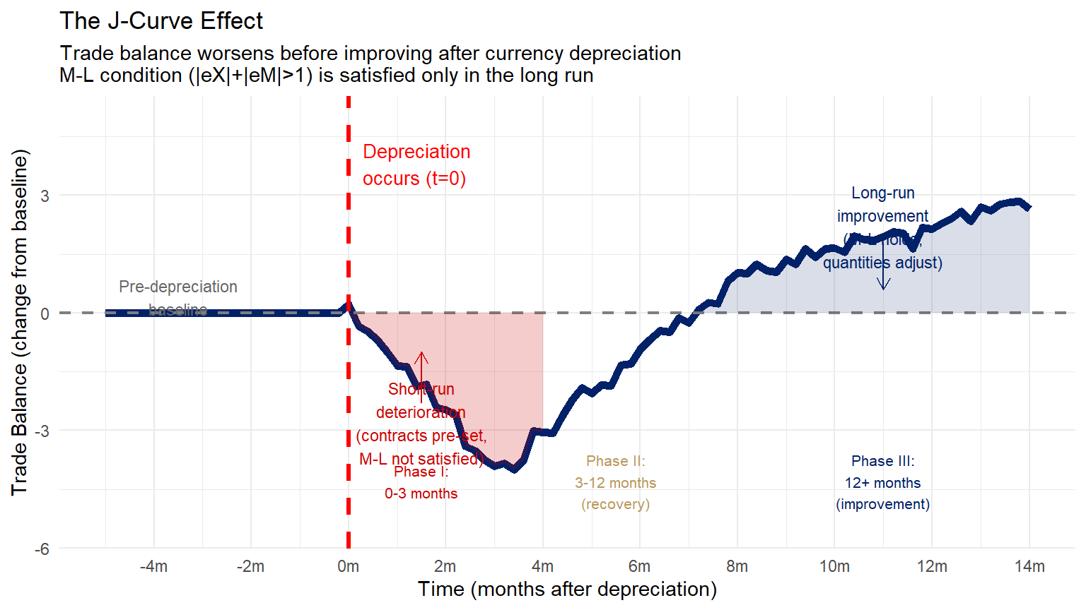
# J-curve shape: initial deterioration then improvement
# TB(t<0) = 0 (baseline)
# After depreciation at t=0:
#   short run (0-3 months): TB falls (pre-set contracts, inelastic demand)
#   medium (3-12 months):   TB recovers as quantities adjust
#   long run (12+ months):  TB improves above baseline if M-L holds

tb_j <- ifelse(
  t < 0, 0,
  ifelse(
    t < 3,
    -4 * (t/3),                                    # deterioration phase
    ifelse(
      t < 8,
      -4 + 5 * ((t - 3)/5),                        # recovery phase
      1 + 0.3 * (t - 8)                             # long-run improvement
    )
  )
)

# Add some noise for realism
tb_j <- tb_j + c(rep(0, sum(t < 0)), rnorm(sum(t >= 0), 0, 0.15))

df <- data.frame(time = t, tb = tb_j)

ggplot(df, aes(x = time, y = tb)) +
  geom_line(color = "#012169", linewidth = 2) +
  geom_hline(yintercept = 0, linetype = "dashed", color = "grey50", linewidth = 0.8) +
  geom_vline(xintercept = 0, linetype = "dashed", color = "red", linewidth = 1.2) +
  # Shaded deterioration region
  geom_ribbon(
    data = df |> filter(time >= 0 & time <= 4),
    aes(ymin = pmin(tb, 0), ymax = 0),
    fill = "#cc0000", alpha = 0.2
  ) +
  # Shaded improvement region
  geom_ribbon(
    data = df |> filter(time > 4),
    aes(ymin = 0, ymax = pmax(tb, 0)),
    fill = "#012169", alpha = 0.15
  ) +
  # Annotations
  annotate("text", x = 0.3, y = 3.8,
           label = "Depreciation\noccurs (t=0)", color = "red", size = 3.5, hjust = 0) +
  annotate("text", x = -3.5, y = 0.4,
           label = "Pre-depreciation\nbaseline", size = 3, color = "grey40") +
  annotate("text", x = 1.5, y = -2.8,
           label = "Short-run\ndeterioration\n(contracts pre-set,\nM-L not satisfied)",
           size = 3, color = "#cc0000", hjust = 0.5) +
  annotate("text", x = 11, y = 2.2,
           label = "Long-run\nimprovement\n(M-L holds,\nquantities adjust)",
           size = 3, color = "#012169", hjust = 0.5) +
  annotate("segment",
           x = 1.5, y = -2.3, xend = 1.5, yend = -1,
           arrow = arrow(length = unit(0.25, "cm")), color = "#cc0000") +
  annotate("segment",
           x = 11, y = 1.8, xend = 11, yend = 0.6,
           arrow = arrow(length = unit(0.25, "cm")), color = "#012169") +
  # Phase labels
  annotate("text", x = 1.5, y = -4.3,
           label = "Phase I:\n0-3 months", size = 2.8, color = "#cc0000") +
  annotate("text", x = 5.5, y = -4.3,
           label = "Phase II:\n3-12 months\n(recovery)", size = 2.8, color = "#B9975B") +
  annotate("text", x = 11,  y = -4.3,
           label = "Phase III:\n12+ months\n(improvement)", size = 2.8, color = "#012169") +
  scale_x_continuous(breaks = seq(-4, 14, 2),
                     labels = paste0(seq(-4, 14, 2), "m")) +
  scale_y_continuous(limits = c(-5.5, 5)) +
  labs(
    title    = "The J-Curve Effect",
    subtitle = "Trade balance worsens before improving after currency depreciation\nM-L condition (|eX|+|eM|>1) is satisfied only in the long run",
    x = "Time (months after depreciation)", y = "Trade Balance (change from baseline)"
  ) +
  theme_minimal(base_size = 11)

Figure 3: J-Curve: Trade Balance Initially Worsens After Currency Depreciation Source: Author’s illustration.

J-curve: mechanisms (3 phases)

• Phase I (0–3 months): contracts fixed → values move before quantities
• Import bill can rise even if volumes don’t
• Phase II (3–12 months): firms adjust sourcing and sales
• Phase III (12+ months): quantities respond fully
• Long run: M–L more likely to hold → TB improves

India: what we see in practice

• 1991: large devaluation; adjustment took time (rigidities)
• 2013: TB improved faster as trade was more integrated
• 2022: oil prices dominated → weaker TB response
• Agriculture adjusts faster than many manufactured goods (more spot pricing)

Absorption approach: policy implication

\[\boxed{CA = Y - A}\quad (A=C+I+G)\]

• Improve CA by raising output (\(Y\)) and/or reducing absorption (\(A\))
• Devaluation helps only if it changes quantities and spending patterns
• Inflation can offset gains if real absorption doesn’t fall

India 1991: adjustment mix

• Fiscal tightening reduced absorption (\(\Delta G<0\))
• Large devaluation switched demand toward domestic goods
• Reforms improved long-run output capacity
• CA improved over time, but growth fell temporarily
• Inflation spiked during adjustment

India’s 1991 BoP crisis: what happened

• Oil prices spiked and external financing dried up (1990–91)
• Forex reserves fell to $5.8B (~3 weeks imports), then $1.2B (~2 weeks)
• India pledged 67 tonnes of gold to raise emergency foreign exchange
• IMF support followed (Aug 1991)
• Adjustment package triggered liberalisation and macro stabilisation

1991 crisis: root causes and policy response

• Fiscal deficit + short-term external borrowing (fragile financing)
• Oil shock (Kuwait crisis) worsened import bill
• Remittance/NRI deposit outflows amplified the squeeze
• Trade liberalisation + industrial delicensing reduced distortions
• FDI opening (automatic route) improved long-run financing

Legacy: the crisis was the proximate cause of India’s 1991 reforms.

India FY2024 BoP Assessment

Current Account:

• CA deficit: $23.2B (-0.7% of GDP) — comfortable
• Merchandise trade deficit: $238B (oil, gold, electronics)
• Services surplus: $163B (IT/BPO dominance)
• Remittances: $120B — world’s largest recipient (World Bank data)

Risks and concerns: (1) Oil price vulnerability: $10/barrel rise adds ~$15B to import bill; (2) FPI volatility: $41B inflow in FY24 could reverse quickly; (3) FDI decline from $55B (FY22) to $22B (FY24) — concerning for long-run financing. India’s CA/GDP (-0.7%) << GDP growth (7%) — external position is sustainable.

Financial Account:

• FDI net inflows: $22B (declined from $83B peak in FY22)
• FPI: +$41B (strong equity market inflows)
• ECB + banking capital: +$25B

Reserve adequacy:

• Forex reserves: $646B (March 2024)
• Import cover: ~11 months (well above IMF 3-month threshold)
• Short-term debt/reserves: 19% (well below 100% danger threshold)

\[\text{CA/GDP} < \text{long-run growth rate} \times \frac{\text{Net foreign debt}}{\text{GDP}}\]

BoP and agriculture: key linkages

• MSP and productivity can reduce food imports (import substitution)
• Export restrictions (rice/onion/sugar) affect credibility and export earnings
• Input policies affect cost competitiveness
• Edible oil dependence is a major import bill risk
• Migration/remittances matter for rural income and the CA

India’s agri trade balance: surplus, with one big weakness

• Net agri balance is typically positive (order of ~$20B)
• Rice and spices are major surplus contributors
• Edible oils are the dominant structural deficit item (≈ -$20B)
• Pulses can be a smaller deficit item in some years

Policy takeaway: edible oils are the macro vulnerability; SPS/processing are the export upside.

India’s services exports: the external-sector cushion

• Services exports create a large surplus (IT/ITES is central)
• They are often more stable than goods exports
• This surplus helps offset the goods trade deficit

Why it matters for policy

• BoP resilience depends heavily on the IT/services engine
• Disruptions to services exports would widen the CA deficit quickly
• Services trade negotiations (Mode 4) are a key Indian interest

Remittances: India’s largest CA credit (FY2024)

• Remittances ≈ $120B (World Bank)
• Major sources: USA, UAE, Saudi Arabia, UK (+ other Gulf)
• Often rise when INR is weaker (more rupees per dollar sent)

Why remittances matter for agriculture

• Smooth consumption during crop shocks
• Finance farm investment (irrigation, equipment, land)
• Enable shift toward higher-value crops (risk capacity)
• Outmigration raises rural wages (labour market effects)
• BoP stabiliser: remittances are large and relatively stable

India’s Forex Reserves: RBI Intervention Chart

reserves_data <- data.frame(
  year      = 2015:2024,
  reserves  = c(341, 360, 370, 424, 412, 477, 590, 633, 578, 646),
  inr_usd   = c(62.1, 65.5, 67.1, 64.5, 69.9, 70.4, 74.2, 75.0, 82.7, 83.3)
)

# Dual-axis plot using secondary axis
coeff <- 10   # scale factor for INR (reserves ~100x INR so scale accordingly

p_res <- ggplot(reserves_data, aes(x = year)) +
  # Reserves bars
  geom_col(aes(y = reserves), fill = "#012169", alpha = 0.75, width = 0.6) +
  # INR/USD line (scaled)
  geom_line(aes(y = inr_usd * coeff), color = "#cc0000", linewidth = 1.5) +
  geom_point(aes(y = inr_usd * coeff), color = "#cc0000", size = 2.5) +
  # Mark 2022 taper tantrum equivalent
  annotate("text", x = 2023, y = 920,
           label = "Post-Ukraine\nrupee weakness\n(₹83/USD)", size = 3, color = "#cc0000") +
  # Mark 2020 reserve build
  annotate("text", x = 2021, y = 650,
           label = "$590B\n(COVID\nreserve build)", size = 3, color = "#012169") +
  scale_x_continuous(breaks = 2015:2024,
                     labels = paste0("FY", substr(2015:2024, 3, 4))) +
  scale_y_continuous(
    name     = "Forex Reserves (USD billion)",
    limits   = c(0, 1000),
    sec.axis = sec_axis(~ . / coeff,
                        name   = "INR per USD",
                        breaks = seq(60, 90, 5))
  ) +
  labs(
    title    = "India's Forex Reserves (bars) and INR/USD Rate (line), FY2015–FY2024",
    subtitle = "RBI builds reserves during capital inflow surges; deploys during stress periods",
    x = NULL
  ) +
  theme_minimal(base_size = 10) +
  theme(
    axis.title.y.right = element_text(color = "#cc0000"),
    axis.text.y.right  = element_text(color = "#cc0000"),
    axis.title.y.left  = element_text(color = "#012169")
  )

p_res

Figure 4: India’s Forex Reserves and INR/USD Exchange Rate, FY2015–FY2024 Source: RBI, Database on Indian Economy (DBIE).

Key Takeaways: Lecture 9

1. National income identity: \(\text{CA} = Y - A = (S - I) + (T - G)\). A CA deficit means the country borrows from abroad — financed by FA inflows or reserve drawdown.

2. BoP accounting: \(\text{CA} + \text{KA} + \text{FA} + \Delta R = 0\). The BoP always balances — surpluses and deficits are in individual accounts, not the overall BoP.

3. India’s external position (FY2024): CA = -0.7% GDP (comfortable); remittances = $120B (world’s largest); services surplus = $163B; forex reserves = $646B (11 months imports). External position is strong.

4. Marshall-Lerner condition: \(|e_X| + |e_M| > 1\) must hold for depreciation to improve TB. In the short run, M-L is typically NOT satisfied → J-curve: TB worsens before improving.

5. India 1991 crisis: Reserves fell to $1.2B (2 weeks imports); India pledged 67 tonnes gold to the BoE. IMF bailout triggered liberalisation — delicensing, trade reform, FDI opening. Crisis → structural reform.

6. Agricultural BoP: India runs a trade surplus in agriculture (~$20B), but edible oil imports (-$21B) are the single largest structural weakness. MSP policy affects both food security and export competitiveness.

Next Lecture Preview

Lecture 10 — Exchange Rates and Agricultural Trade June 27, 2026

• Fixed vs flexible exchange rate systems
• Purchasing Power Parity (PPP): absolute and relative
• Real exchange rate: \(q = eP^*/P\) and agricultural competitiveness
• How rupee depreciation affects Indian rice and wheat exports
• Dutch disease: can commodity booms harm agricultural exporters?

• India’s managed float: RBI intervention and the REER

Preparation: Review Salvatore Ch. 14–15 (Exchange Rates). Note that India operates a managed float — this means understanding both PPP theory AND RBI’s intervention behaviour. We will use regression analysis of real exchange rate and export volume data.

Appendix

Additional Resources

Further reading

• Salvatore, International Economics (relevant chapters)
• Appleyard & Field, International Economics (relevant chapters)

Key data sources

• DGCI&S: merchandise trade
• RBI: balance of payments
• APEDA: agricultural export statistics
• WTO: tariff + trade databases