Lecture 8: Protectionism II — Subsidies, Dumping & Cartels

Econ 2203 | International Trade and Policy in Agriculture

Nithin M

Department of Development Economics

2026-06-13

Recap: Tariffs and Quotas

Last lecture (L7): border instruments that restrict imports

Tariffs → raise domestic price $P_d = P_w(1+t)$, generate revenue $t \cdot M$, DWL $= b + d$
Quotas → fix import volume $\bar{M}$; quota rents go to licence holders
India: high bound tariffs, TRQs, tariff “water” provides policy flexibility

Today: instruments that push exports or distort domestic production: export subsidies, dumping, VERs, and cartels.

Political economy insight: Tariffs/quotas protect import-competing producers. Export subsidies protect exporting producers. Both are driven by producer lobbying — even though consumers and taxpayers bear the cost: $\text{Producer surplus gain} > \text{Consumer + taxpayer loss?}$ — usually no in aggregate, but politically organised producers win.

What Is an Export Subsidy?

An export subsidy is a direct government payment $s$ per unit exported.

Mechanism: Domestic producers can sell abroad at $P_w$ and receive subsidy $s$, so net return = $P_w + s$ → domestic price rises to $P_d = P_w + s$.

Group	Direction	Why
Producers	Gain	Higher domestic price
Consumers	Lose	Pay $P_d > P_w$
Government	Pays	$s \times \text{export volume}$

Price wedge identity: $\boxed{P_d = P_w + s}$; $Q_s \uparrow$, $Q_d \downarrow$, Exports $= Q_s - Q_d \uparrow$

Large-country effect: World price $P_w$ falls as export supply increases → terms of trade deteriorate → exporter loses even more: $\Delta W_{\text{large country}} < \Delta W_{\text{small country}} < 0$

Export Subsidy: Welfare Diagram

Show R code

# D: P = 50 - 0.5Q  =>  Qd = 100 - 2P
# S: P = 5  + 0.5Q  =>  Qs = 2P - 10
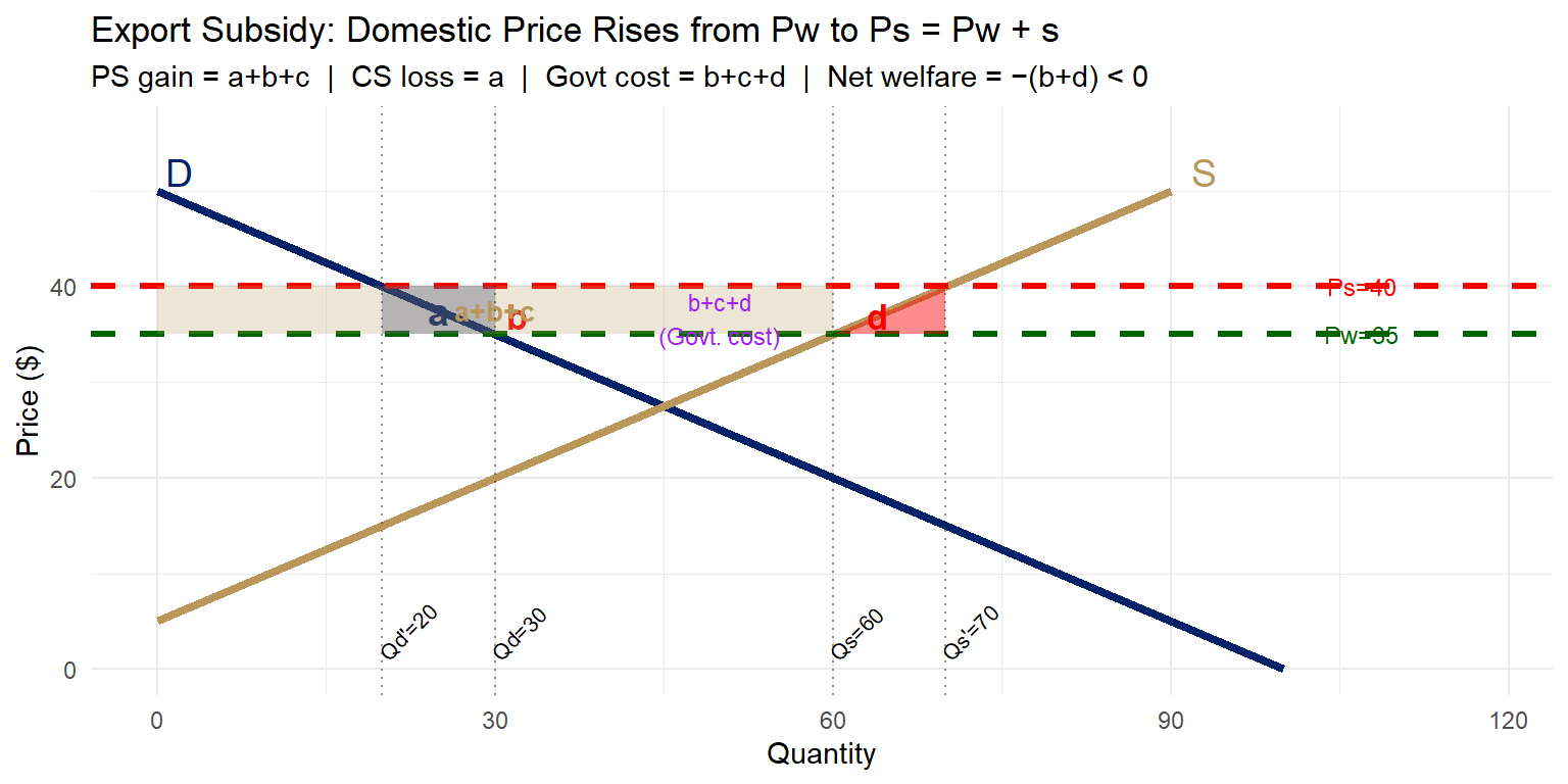
# Autarky equilibrium: P=27.5, Q=45
# World price Pw=35 (country has comparative advantage, exports)
# At Pw=35: Qd=30, Qs=60, Exports=30
# Subsidy s=5 raises domestic price to Ps=40
# At Ps=40: Qd=20, Qs=70, Exports=50

Pw <- 35; s <- 5; Ps <- Pw + s
Qd0 <- 100 - 2*Pw   # 30  (domestic consumption before subsidy)
Qs0 <- 2*Pw - 10    # 60  (domestic supply before subsidy)
Qd1 <- 100 - 2*Ps   # 20  (domestic consumption after subsidy)
Qs1 <- 2*Ps - 10    # 70  (domestic supply after subsidy)

# Welfare areas
# a  = CS loss (rectangle): (Ps-Pw)*(Qd0-Qd1) = 5*10 = 50
# b  = DWL consumption triangle: 0.5*(Ps-Pw)*(Qd0-Qd1) = 25  [already in a's triangle portion]
# Actually: a = full rectangle between Qd1 and Qd0; b = triangle at Qd0 end
# Standard labeling (Salvatore style):
# a = rectangle: Pw to Ps, Qd1 to Qd0 = 5*10=50
# b = triangle (consumption DWL): 0.5*5*10 = 25 -- but let's use numeric polygon

ggplot() +
  # ── curves ───────────────────────────────────────────────────────────────────
  geom_segment(aes(x = 0,  y = 50, xend = 100, yend = 0),
               color = "#012169", linewidth = 1.5) +           # Demand
  geom_segment(aes(x = 0,  y = 5,  xend = 90,  yend = 50),
               color = "#B9975B", linewidth = 1.5) +           # Supply
  # ── price lines ──────────────────────────────────────────────────────────────
  geom_hline(yintercept = Pw, linetype = "dashed",
             color = "darkgreen", linewidth = 1.2) +
  geom_hline(yintercept = Ps, linetype = "dashed",
             color = "red",       linewidth = 1.2) +
  # ── area a: CS loss rectangle (Qd1→Qd0, Pw→Ps) ──────────────────────────────
  annotate("polygon",
           x = c(Qd1, Qd0, Qd0, Qd1),
           y = c(Pw,  Pw,  Ps,  Ps),
           fill = "#012169", alpha = 0.30) +
  annotate("text", x = (Qd1+Qd0)/2, y = (Pw+Ps)/2,
           label = "a", size = 5, fontface = "bold", color = "#012169") +
  # ── area b: DWL consumption triangle ─────────────────────────────────────────
  annotate("polygon",
           x = c(Qd1, Qd0, Qd1),
           y = c(Ps,  Pw,  Ps),
           fill = "red", alpha = 0.45) +
  annotate("text", x = Qd0 + 2, y = Pw + 2,
           label = "b", size = 4.5, color = "red", fontface = "bold") +
  # ── area a+b+c: PS gain (0→Qs0, Pw→Ps rectangle) ────────────────────────────
  annotate("polygon",
           x = c(0,   Qs0, Qs0, 0),
           y = c(Pw,  Pw,  Ps,  Ps),
           fill = "#B9975B", alpha = 0.25) +
  annotate("text", x = Qs0/2, y = (Pw+Ps)/2,
           label = "a+b+c", size = 3.5, fontface = "bold", color = "#B9975B") +
  # ── area d: DWL production triangle (Qs0→Qs1, Pw→Ps) ────────────────────────
  annotate("polygon",
           x = c(Qs0, Qs1, Qs1),
           y = c(Pw,  Pw,  Ps),
           fill = "red", alpha = 0.45) +
  annotate("text", x = Qs0 + 4, y = Pw + 2,
           label = "d", size = 4.5, color = "red", fontface = "bold") +
  # ── govt cost label ──────────────────────────────────────────────────────────
  annotate("text", x = (Qd1+Qs1)/2 + 5, y = (Pw+Ps)/2 - 0.8,
           label = "b+c+d\n(Govt. cost)", size = 3, color = "purple") +
  # ── vertical reference lines ─────────────────────────────────────────────────
  geom_vline(xintercept = c(Qd1, Qd0, Qs0, Qs1),
             linetype = "dotted", alpha = 0.4) +
  annotate("text", x = Qd1, y = 1.5,
           label = paste0("Qd'=", Qd1), size = 2.8, angle = 45, hjust = 0) +
  annotate("text", x = Qd0, y = 1.5,
           label = paste0("Qd=",  Qd0), size = 2.8, angle = 45, hjust = 0) +
  annotate("text", x = Qs0, y = 1.5,
           label = paste0("Qs=",  Qs0), size = 2.8, angle = 45, hjust = 0) +
  annotate("text", x = Qs1, y = 1.5,
           label = paste0("Qs'=", Qs1), size = 2.8, angle = 45, hjust = 0) +
  annotate("text", x = 107, y = Pw,
           label = paste0("Pw=", Pw), size = 3.2, color = "darkgreen") +
  annotate("text", x = 107, y = Ps,
           label = paste0("Ps=", Ps), size = 3.2, color = "red") +
  annotate("text", x = 2,  y = 52, label = "D", size = 5, color = "#012169") +
  annotate("text", x = 93, y = 52, label = "S", size = 5, color = "#B9975B") +
  scale_x_continuous(limits = c(0, 118)) +
  scale_y_continuous(limits = c(0, 56)) +
  labs(
    title    = "Export Subsidy: Domestic Price Rises from Pw to Ps = Pw + s",
    subtitle = "PS gain = a+b+c  |  CS loss = a  |  Govt cost = b+c+d  |  Net welfare = −(b+d) < 0",
    x = "Quantity", y = "Price ($)"
  ) +
  theme_minimal(base_size = 11)

Figure 1: Export Subsidy: Welfare Analysis for the Exporting Country Source: Author’s illustration.

Welfare Accounting: Export Subsidy

Full decomposition (exporting country, small-country case):

\[\Delta CS = -a \qquad \Delta PS = +(a + b + c) \qquad \text{Government cost} = -(b + c + d)\]

\[\boxed{\Delta W = -(b + d) < 0}\]

$b$ = consumption distortion triangle; $d$ = production distortion triangle

Govt cost = $s \times (Q_{s1} - Q_{d1})$ = $5 \times 50 = 250$ units

Numerical check:

Area	Formula	Value
$a$	$5 \times 10$	50
$b$	$\frac{1}{2} \times 5 \times 10$	25
$c$	$5 \times (60-30)$	150
$d$	$\frac{1}{2} \times 5 \times 10$	25

$\Delta W = -(b+d) = -(25+25) = -50$; Govt pays: $(b+c+d) = 200$; PS gains: $(a+b+c) = 225$; CS loses: $a = 50$

India’s Export Subsidies: Sugar Case (WTO DS579)

Background: India’s sugar support involves: SMP (Statutory Minimum Price); FRP (Fair and Remunerative Price); production assistance subsidy (₹13.88/quintal); MIEQ (mandated minimum export quota); transport subsidy (₹1,000/tonne).

WTO DS579 (2019): Brazil, Australia, Guatemala challenged India. 2021 Panel ruling: India’s domestic support and export subsidies exceeded WTO AoA commitments. India appealed → pending (Appellate Body non-functional since 2019).

India’s defence: “Developing countries have the right to support food security and rural livelihoods.”

AoA de minimis provision: Amber Box support ≤ 10% of production value
Peace Clause for public stockholding; Special and Differential Treatment (SDT)

Market impact: India’s subsidised sugar exports depress world prices by an estimated 3–7% — harming Brazil, Thailand, and African sugar exporters.

MSP, FCI, and the Peace Clause

MSP mechanism: CACP recommends MSP for 23 crops pre-season; FCI/NAFED/CCI procure at MSP when market falls below; surplus procured stock → sometimes exported.

WTO problem: If $\text{MSP} > P_w$ and surplus exported at $P_w$: $\text{Implicit subsidy} = (\text{MSP} - P_w) \times Q_{\text{exported}}$

	MSP	World price	Implicit subsidy
Rice	$290	$450	—
Wheat	$245	$260	~$15/t

Bali Peace Clause (2013): WTO members agreed not to legally challenge food security stockholding programmes of developing countries — even if support exceeds 10% AMS limit. Condition: transparency + no trade distortion.

Nairobi (2015) → MC13 Abu Dhabi (2024): Permanent solution still pending. India insists on a permanent peace clause without the non-distortion condition. USA/EU resist — argue India’s 800M tonne/year FCI operations are massively trade-distorting. High-stakes stalemate.

What Is Dumping? Formal Definition

WTO Anti-Dumping Agreement (Article 2): Dumping occurs when the export price is below normal value:

\[\text{Normal value} = \begin{cases} P_d & \text{(home market price)} \\ P_{3C} & \text{(price to third country)} \\ COP + \text{profit} & \text{(constructed value)} \end{cases}\]

\[\text{Margin of dumping} = \text{Normal value} - P_x > 0\]

Three conditions to impose anti-dumping duty: (1) Dumping margin > 0 (threshold: >2%); (2) material injury (or threat) to domestic industry; (3) causal link between dumping and injury.

Why would a firm dump? Price discrimination (monopoly at home, competitive abroad); predatory intent (eliminate competition); surplus disposal; learning curve; input subsidy pass-through.

Dumping ≠ comparative advantage: Genuinely lower costs look like dumping when compared to high-cost domestic producers.

Types of Dumping

1. Sporadic Dumping: Occasional disposal of excess inventory at below-normal price. India example: Bumper harvest years → surplus wheat exported below MSP procurement price. Welfare effect on importer: Minor, temporary.

2. Predatory Dumping: Strategic pricing to eliminate foreign competition, then raise prices once rivals exit. Classic allegation: Chinese steel exports to India (2014–16). HRC steel exported at $350/tonne vs cost of $450. Welfare effect: Temporary gain, long-run monopolisation.

3. Persistent Dumping: Chronic price discrimination — domestic market protected → monopoly pricing at home; competitive pricing abroad: $P_d > P_x$ persistently.

Arbitrage prevention: For persistent dumping to work, the exporter must prevent re-importation of cheaply sold exports back into the home market. Methods: different packaging, branding, warranty restrictions, official import controls.

Dumping: Price Discrimination Diagram

Show R code

# Domestic market: inelastic demand, protected → high monopoly price
p1 <- ggplot() +
  # Demand (steep = inelastic)
  geom_segment(aes(x = 0, y = 60, xend = 60, yend = 0),
               color = "#012169", linewidth = 1.5) +
  # MC = Supply
  geom_segment(aes(x = 0, y = 10, xend = 80, yend = 50),
               color = "#B9975B", linewidth = 1.5) +
  # MR (derived from P = 60 - Q  =>  MR = 60 - 2Q)
  geom_segment(aes(x = 0, y = 60, xend = 30, yend = 0),
               color = "#012169", linewidth = 1, linetype = "dashed") +
  # Monopoly price Pd=40, Qd=20: MC=10+Q/2=10+10=20... let's use P=40
  geom_hline(yintercept = 40, linetype = "dashed", color = "red", linewidth = 1) +
  geom_vline(xintercept = 20, linetype = "dotted", color = "grey50") +
  annotate("point", x = 20, y = 40, size = 3, color = "red") +
  annotate("text", x = 26, y = 41,
           label = "Monopoly\nequilibrium\nPd = 40", size = 2.8, color = "red") +
  annotate("text", x =  2, y = 62, label = "D",  size = 4, color = "#012169") +
  annotate("text", x =  2, y = 57, label = "MR", size = 3.5, color = "#012169",
           fontface = "italic") +
  annotate("text", x = 82, y = 52, label = "MC", size = 4, color = "#B9975B") +
  scale_x_continuous(limits = c(0, 88), breaks = seq(0, 80, 20)) +
  scale_y_continuous(limits = c(0, 65)) +
  labs(title = "Domestic Market",
       subtitle = "Protected market → high price (Pd = 40)",
       x = "Quantity", y = "Price ($)") +
  theme_minimal(base_size = 10)

# Export market: elastic demand (world price = horizontal demand)
p2 <- ggplot() +
  # Horizontal world demand (perfectly elastic)
  geom_hline(yintercept = 25, color = "#012169", linewidth = 1.5) +
  # MC
  geom_segment(aes(x = 0, y = 10, xend = 80, yend = 50),
               color = "#B9975B", linewidth = 1.5) +
  # Export price (below domestic price)
  geom_hline(yintercept = 25, linetype = "dashed", color = "darkgreen", linewidth = 1) +
  # MC = Px at Q=30: 10 + 0.5*30 = 25
  geom_vline(xintercept = 30, linetype = "dotted", color = "grey50") +
  annotate("point", x = 30, y = 25, size = 3, color = "darkgreen") +
  annotate("text", x = 35, y = 26,
           label = "Export eq.\nPx = 25 < Pd = 40\nDUMPING!", size = 2.8, color = "darkgreen") +
  annotate("text", x =  2, y = 27, label = "D* (world price)", size = 3.5, color = "#012169") +
  annotate("text", x = 82, y = 52, label = "MC", size = 4, color = "#B9975B") +
  scale_x_continuous(limits = c(0, 88), breaks = seq(0, 80, 20)) +
  scale_y_continuous(limits = c(0, 65)) +
  labs(title = "Export Market",
       subtitle = "Competitive market → Px = Pw = 25 < Pd",
       x = "Quantity", y = "Price ($)") +
  theme_minimal(base_size = 10)

p1 + p2 +
  plot_annotation(
    title    = "Dumping: Price Discrimination Between Domestic and Export Markets",
    subtitle = "Condition: (a) home market more inelastic than export market; (b) import barriers prevent arbitrage\nDumping margin = Pd − Px = 40 − 25 = $15 per unit",
    theme = theme_minimal(base_size = 11)
  )

Figure 2: Dumping as Price Discrimination: Domestic Monopoly Price > Export Price Source: Author’s illustration.

Dumping: Formal Condition and Anti-Dumping Duty

Dumping condition (price discrimination version):

\[P_x < P_d \quad \Leftrightarrow \quad \frac{P_x}{P_d} < 1\]

In profit-maximising terms: $P_d \left(1 - \frac{1}{|e_d|}\right) = P_x \left(1 - \frac{1}{|e_x|}\right)$

If $|e_x| > |e_d|$ (export market more elastic), then $P_x < P_d$. ✓

Anti-dumping duty (ADD): $\text{ADD} = P_d - P_x = \text{margin of dumping}$ — raises $P_x$ back toward $P_d$.

Welfare effects of ADD for importing country:

Effect	Direction
Consumer surplus	Falls (price rises)
Producer surplus	Rises (domestic producers protected)
Govt revenue (ADD)	Rises
Net welfare	Ambiguous — DWL likely

$\Delta W = -b - d + \text{PS gain}$ — if domestic production is efficient, $\Delta W$ may be positive; if ADD is protectionist, $\Delta W < 0$.

India’s Anti-Dumping Experience

Show R code

ad_data <- data.frame(
  sector = c("Chemicals &\nPetrochemicals", "Steel &\nMetals", "Textiles &\nFibres",
             "Rubber &\nPlastics", "Machinery &\nEquipment", "Agriculture\n& Food"),
  investigations = c(42, 38, 22, 18, 12, 8),
  top_source      = c("China", "China/EU", "China", "China/Korea", "China/EU", "China/Myanmar")
)
ad_data <- ad_data |>
  arrange(investigations) |>
  mutate(sector = factor(sector, levels = sector))

ggplot(ad_data, aes(x = sector, y = investigations)) +
  geom_col(fill = "#012169", width = 0.65) +
  geom_text(aes(label = investigations), hjust = -0.25, size = 3.8,
            fontface = "bold", color = "#012169") +
  coord_flip() +
  scale_y_continuous(limits = c(0, 52), expand = c(0, 0)) +
  labs(
    title    = "India's Anti-Dumping Investigations by Sector, 2015–2024",
    subtitle = "India is the world's largest user of anti-dumping measures (WTO data)\nPrimary target: China in nearly all sectors",
    x = NULL, y = "Number of AD Investigations"
  ) +
  theme_minimal(base_size = 11) +
  theme(panel.grid.major.y = element_blank())

Figure 3: India: Anti-Dumping Investigations Initiated by Sector (2015–2024) Source: DGTR, Ministry of Commerce, GoI.

Indian Agriculture Facing Dumping Allegations Abroad

Indian shrimp exports (USA): USA imposed CVD + AD duties on Indian shrimp (2003, 2013, 2023); margin of dumping: 4.98–6.3% (2023 review). India’s argument: low costs reflect genuine comparative advantage (labour, aquaculture efficiency), not subsidies.

Indian basmati rice: EU phytosanitary restrictions (pesticide MRLs) periodically block Indian exports — not formal AD, but equivalent effect.

Indian buffalo meat: EU AD allegations (cold cuts); AD margin investigations initiated 2021. India’s position: lowest-cost producer due to cattle by-product economics.

Comparative advantage vs. dumping: A developing country with genuinely low costs will appear to dump when compared to high-cost producers in developed countries. $P_{\text{India}} < P_{\text{USA}} \not\Rightarrow \text{dumping}$. Dumping requires $P_{\text{export}} < \text{normal value}$. In practice, AD is often used as disguised protectionism.

VERs — Quotas Imposed “Voluntarily” by Exporters

A Voluntary Export Restraint (VER) is an agreement where the exporting country “voluntarily” limits its exports — usually under diplomatic pressure.

Why “voluntary”? Importing country threatens worse action; exporter prefers VER — quota rent goes to foreign exporter; both governments prefer quiet bilateral deal to WTO dispute.

Classic example: Japan–USA auto VER (1981): Japan agreed to limit car exports at 1.68M units/year. Toyota, Honda captured quota rent → funded quality upgrading → ultimately made Japanese cars stronger.

VER vs. Tariff vs. Quota:

Instrument	Who gets rent?	WTO-legal?
Tariff	Importing govt	Yes
Quota	Licence holders	Yes (with rules)
VER	Foreign exporter	No (UR banned)

Uruguay Round (1994): VERs explicitly prohibited under WTO safeguards agreement. But “Orderly Marketing Arrangements” and “grey area” bilateral deals persist under different names.

VER Welfare Analysis

A VER is economically equivalent to an import quota — but worse for the importing country:

Standard quota welfare: $\Delta W_{\text{import country}} = -(b + d) + c$ where $c$ = quota rent captured by licence holders.

VER welfare: $\Delta W_{\text{import country}} = -(b + c + d)$ because $c$ = quota rent goes to foreign exporters, not domestic licence holders.

\[\boxed{\text{VER strictly worse than equivalent quota for importing country}}\]

Numerical example: Suppose VER restricts imports to $\bar{M}$.

$b$ = production distortion: $\frac{1}{2}(P_d - P_w) \cdot \Delta Q_s$
$c$ = quota rent: $(P_d - P_w) \cdot \bar{M}$
$d$ = consumption distortion: $\frac{1}{2}(P_d - P_w) \cdot \Delta Q_d$

Under tariff: $\Delta W_{\text{tariff}} = -(b+d) + t \cdot M$; Under VER: $\Delta W_{\text{VER}} = -(b+c+d) < \Delta W_{\text{tariff}}$

What Is a Cartel? Conditions for Success

A cartel is a formal/informal agreement among producers to restrict output, fix prices, or divide markets. Profit-maximising cartel acts as a monopolist: $MR = MC \Rightarrow Q^* < Q_{\text{competitive}}, P^* > P_{\text{competitive}}$; world welfare loss = $-(b + d)$.

Conditions for cartel success: (1) Concentrated supply; (2) inelastic demand; (3) discipline (no cheating); (4) barriers to entry; (5) product homogeneity.

OPEC as reference: OPEC controls ~38% of world oil supply. Production cuts (2022–23) raised Brent crude from $75 to $120/barrel.

Agricultural cartels rarely succeed: Many producers; many substitutes (rice ↔︎ wheat ↔︎ maize); perishable goods; low entry barriers; political pressure to sell for domestic food security.

\[\Rightarrow \text{Agricultural cartels are theoretically possible, practically unstable}\]

International Commodity Agreements (ICAs): instruments

ICAs are multilateral attempts to stabilise commodity prices.

Buffer stocks: buy when price is “too low”, sell when “too high”
Export quotas: allocate export shares across members
Long-term contracts: guarantee volumes at agreed prices
Works best when: large market share, homogeneous commodity, credible financing
Key caution: agriculture has close substitutes → stability is hard

Why ICAs fail in practice

Free-rider problem: non-members expand exports when prices rise
Cheating: members secretly exceed quotas
Financing constraint: buffer stocks become fiscally unsustainable
Substitutes + tech change: demand shifts undermine price bands
North–South conflict: producers want high prices; consumers want low prices

History of International Commodity Agreements

Examples and outcomes:

Coffee (ICO): collapsed (free-riding)
Tin (ITA): collapsed (buffer-stock bankruptcy)
Sugar (ISA): weakened (price provisions abandoned)
Jute (IJO): wound down (2014)
Cocoa (ICCO): repeated failures; restructured

Tin crisis (1985): why buffer stocks fail

Prices fell sharply; buffer-stock manager ran out of funds
Agreement collapsed and disrupted the tin market
Prices plunged by about 40% in days
Price bands require credible financing (hard politically)
Takeaway: ICAs are fragile when compliance and funding are weak

India’s Rice Export Ban (2023): Unilateral Market Power

India’s rice export market position:

World’s largest rice exporter: ~40% of global rice trade (FY2022-23: 22 MMT)
Dominant in non-basmati white rice: ~60% of world market

August 2023 policy actions:

Ban on non-basmati white rice exports
20% export duty on parboiled rice
$1,200/tonne MEP on basmati rice

Immediate market impact:

World rice prices surged 20–30% in 2 months
Philippines, Indonesia, West Africa most affected
Bangladesh, Senegal faced acute food security risks

Economic analysis:

With 40% world market share, India has significant monopsonist/monopolist power in rice — analogous to a cartel without formal coordination.

India’s justification: WTO Article XI permits export restrictions for food security.

Counter-argument: When a single country controls 40% of world supply, its “domestic food security” restriction is a global food security threat.

\[P_{\text{world}} \uparrow 25\% \Rightarrow \text{500M+ people in importing countries pay more for food}\]

Lesson: Market concentration creates policy power — with global externalities.

Strategic Trade Policy and Infant Industry Argument

Infant industry argument (Hamilton 1791; List 1841):

Temporary protection allows a new industry to: 1. Achieve economies of scale 2. Move down the learning curve 3. Become internationally competitive

Learning-by-doing model:

\[C_t = C_0 \cdot e^{-\lambda Q_t^{\text{cumulative}}}\]

where $\lambda$ = learning rate. Production cost falls with cumulative experience.

Protection justified if:

\[\sum_{t=0}^{T} \frac{\text{PS gain}_t - \text{CS loss}_t}{(1+r)^t} > 0\]

i.e., present value of future gains exceeds current protection costs.

India examples:

Edible oil (1970s-90s): Heavy protection of domestic oilseed processing. - Result: Yellow revolution (oilseed production rose) - But productivity gains lagged; protection lasted too long

Sugar industry: - 100+ years of protection - Still high-cost producer by global standards - Protection → no incentive to compete

Counter-argument to infant industry: If the learning curve is genuinely valuable, private capital should finance it. Government intervention needed only if: (a) capital market failure, or (b) positive spillovers (externalities) that private firm cannot capture.

\[\text{Subsidy justified} \iff \text{market failure exists}\]

WTO Disciplines: Key Rules Summary

Instrument	WTO status
Export subsidies (developed)	Prohibited (MC10 Nairobi 2015)
Export subsidies (developing)	Phased out
Domestic subsidies (Amber Box)	Limited by AMS cap
Anti-dumping duties	Permitted (ADA)
Countervailing duties	Permitted (SCMA)
VERs	Prohibited (Art. 11, SA)
Export restrictions (quotas/bans)	Permitted for food security (Art. XI:2)
Export cartels	No explicit WTO rule — governed by domestic competition law

Countervailing Duties (CVD):

CVDs target foreign subsidies (not dumping):

\[\text{CVD} = \text{amount of foreign subsidy}\]

Condition: subsidy is “specific” (to a firm/industry) AND causes material injury.

SCMA Agreement governs CVDs.

India has faced CVDs primarily from USA on shrimp, steel, and pharmaceutical exports.

India has used CVDs less frequently than AD duties — but use is growing as India targets subsidised Chinese and EU agricultural exports.

Key Takeaways: Lecture 8

1. Export subsidies distort production and trade; harm importing-country farmers; impose fiscal costs on the subsidising government. Net welfare effect for exporting country: $\Delta W = -(b+d) < 0$.

2. India’s MSP + FCI procurement creates implicit export subsidies when procurement prices exceed world prices. Sugar WTO dispute (DS579) shows WTO’s limits in disciplining developing country support.

3. Dumping = selling below normal value. Formal condition: $P_x < P_d$ or $P_x < AVC$. India is the world’s largest AD user; but Indian exporters also face spurious AD allegations that confuse genuine comparative advantage with dumping.

4. VERs are strictly worse than equivalent tariffs for the importing country — quota rent is transferred abroad: $\Delta W_{\text{VER}} = -(b+c+d) < -(b+d) = \Delta W_{\text{tariff}}$.

5. Agricultural cartels fail because: many producers, many substitutes, perishable goods, easy entry. But India’s unilateral market power in rice (40% of world exports) achieves cartel-like effects without formal coordination.

Next Lecture Preview

Lecture 9 — Balance of Trade & Balance of Payments June 20, 2026

What is the BoP? Three-account structure and accounting identity
National income identity approach: $\text{CA} = Y - A = S - I + (T - G)$
India’s current account: merchandise deficit, services surplus, remittances
Capital and financial account: FDI vs FPI, RBI reserve management
Marshall-Lerner condition: $|e_X| + |e_M| > 1$

Appendix

Additional Resources

Further Reading

International Economics — Salvatore (Ch. 9-11)
International Economics — Appleyard & Field (Ch. 9-11)
RBI/DGCI&S/APEDA databases for latest data

Key Data Sources

DGCI&S: India’s merchandise trade
RBI: Balance of payments data
APEDA: Agricultural export statistics
WTO: Tariff and trade databases

Area	Formula	Value
\(a\)	\(5 \times 10\)	50
\(b\)	\(\frac{1}{2} \times 5 \times 10\)	25
\(c\)	\(5 \times (60-30)\)	150
\(d\)	\(\frac{1}{2} \times 5 \times 10\)	25