Lecture 7: Protectionism I — Tariffs & Quotas

Econ 2203 | International Trade and Policy in Agriculture

Nithin M

Department of Development Economics

2026-06-06

Recap: Free Trade and Its Limits

Comparative advantage says free trade maximises global welfare:

• Resources flow to most efficient uses
• Both countries gain from specialisation
• Prices converge across borders

But reality differs: Most countries protect agriculture. India levies average tariffs of ~36% on farm goods. Why?

Today’s question: When — if ever — is protection economically justified?

Overview of Protectionist Instruments

Instrument	Mechanism	Example
Tariff	Tax on imports	India palm oil duty 100%
Quota	Quantity limit	TRQ on wheat
Export subsidy	Payment to exporters	US Farm Bill
Anti-dumping duty	Penalty for below-cost pricing	India vs Chinese garlic
NTB / SPS / TBT	Standards, labelling, sanitary rules	Pesticide MRLs
VER	Exporter self-limits	Japan autos to USA

Lectures 7–8 cover each instrument in turn. NTBs revisited in Lecture 15.

The Case for Protection

Six main arguments:

1. Infant industry — temporary protection allows domestic industry to reach scale
2. Food security / national security — strategic self-sufficiency
3. Employment protection — preserve rural livelihoods
4. Optimal tariff — large-country terms-of-trade argument
5. Revenue — government finances via import duties
6. Anti-dumping — level the playing field against predatory foreign pricing

Economic validity: Infant industry and optimal tariff have theoretical foundations. Employment, revenue, and food security are political economy arguments — valid as policy goals but do not imply trade restriction is the best tool.

What is a Tariff?

A tariff is a tax levied on imported goods at the border.

Types:

• Specific tariff: fixed amount per unit (e.g. ₹500 per tonne of wheat)
• Ad valorem tariff: percentage of import value (e.g. 50% on wheat)
• Compound tariff: specific + ad valorem combined

India uses primarily ad valorem tariffs across agricultural commodities.

Effect of a tariff: \(P_{domestic} = P_{world} + t\)

Domestic price rises → domestic production rises → imports fall → consumer surplus falls → government earns revenue

Baseline: Free Trade Welfare

Pw <- 15
Pautarky <- 30

ggplot() +
  geom_segment(aes(x=0, y=50, xend=100, yend=0), color="#012169", linewidth=1.5) +
  geom_segment(aes(x=0, y=10, xend=80, yend=50), color="#B9975B", linewidth=1.5) +
  geom_hline(yintercept=Pw, linetype="dashed", color="darkgreen", linewidth=1.2) +
  annotate("polygon", x=c(0,0,70), y=c(50,15,15), fill="#012169", alpha=0.15) +
  annotate("polygon", x=c(0,10,0), y=c(10,15,15), fill="#B9975B", alpha=0.3) +
  geom_vline(xintercept=10, linetype="dotted", color="#B9975B") +
  geom_vline(xintercept=70, linetype="dotted", color="#012169") +
  annotate("text", x=10, y=3, label="Qs=10", size=3.5, color="#B9975B") +
  annotate("text", x=70, y=3, label="Qd=70", size=3.5, color="#012169") +
  annotate("text", x=102, y=0, label="D", size=4, color="#012169") +
  annotate("text", x=82, y=50, label="S", size=4, color="#B9975B") +
  annotate("text", x=105, y=Pw, label=paste0("Pw = ", Pw), size=3.5, color="darkgreen") +
  annotate("text", x=35, y=35, label="CS", size=5, color="#012169", fontface="bold") +
  annotate("text", x=5, y=13, label="PS", size=3.5, color="#B9975B", fontface="bold") +
  annotate("text", x=40, y=12, label="Imports = 60", size=3.5, color="darkgreen") +
  scale_x_continuous(limits=c(0,110), breaks=seq(0,100,20)) +
  scale_y_continuous(limits=c(0,55), breaks=seq(0,50,10)) +
  labs(title="Free Trade Equilibrium",
       subtitle="At world price Pw=15: Qs=10, Qd=70, Imports=60",
       x="Quantity", y="Price (₹/unit)") +
  theme_minimal(base_size=11)

Figure 1: Free Trade: Domestic Supply, Demand, and World Price Source: Author’s illustration.

Free trade baseline: \(D: P = 50 - Q/2\) · \(S: P = 10 + Q/2\) · \(P_w = 15\)

At \(P_w=15\): domestic supply \(Q_s=10\), domestic demand \(Q_d=70\), imports = 60 units.

Partial Equilibrium Analysis of a Tariff

Free trade equilibrium at \(P_w\): Domestic supply \(Q_s^0\); domestic demand \(Q_d^0\); imports \(M_0 = Q_d^0 - Q_s^0\)

After tariff \(t\): domestic price → \(P_w + t\): Domestic supply rises: \(Q_s^1 > Q_s^0\); demand falls: \(Q_d^1 < Q_d^0\); imports fall: \(M_1 = Q_d^1 - Q_s^1 < M_0\)

Welfare triangles:

Effect	Direction
Consumer surplus	↓ (trapezoid A+B+C+D)
Producer surplus	↑ (rectangle A)
Govt revenue	↑ (rectangle C)
Deadweight loss	↑ (triangles B + D)

Triangle B = production distortion loss (resources diverted to inefficient domestic production)

Triangle D = consumption distortion loss (consumers priced out of market)

Both are pure efficiency loss.

Effect of a Tariff — Welfare Analysis

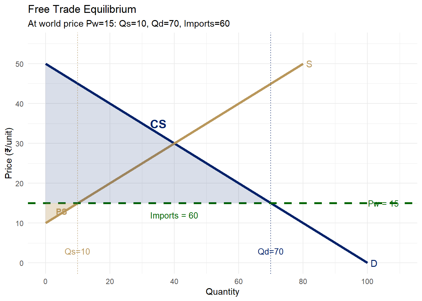
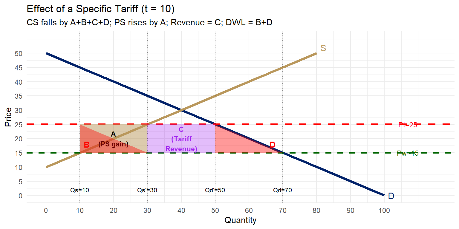
Pw <- 15; t <- 10; Pt <- Pw + t

Qd_free   <- 100 - 2*Pw   # 70
Qs_free   <- -20 + 2*Pw   # 10
Qd_tariff <- 100 - 2*Pt   # 50
Qs_tariff <- -20 + 2*Pt   # 30

ggplot() +
  geom_segment(aes(x=0, y=50, xend=100, yend=0), color="#012169", linewidth=1.5) +
  geom_segment(aes(x=0, y=10, xend=80, yend=50), color="#B9975B", linewidth=1.5) +
  geom_hline(yintercept=Pw, linetype="dashed", color="darkgreen", linewidth=1) +
  geom_hline(yintercept=Pt, linetype="dashed", color="red", linewidth=1.2) +
  # Area A: PS gain rectangle
  annotate("polygon", 
           x=c(Qs_free, Qs_tariff, Qs_tariff, Qs_free), 
           y=c(Pw, Pw, Pt, Pt), 
           fill="#B9975B", alpha=0.5) +
  annotate("text", x=(Qs_free+Qs_tariff)/2, y=(Pw+Pt)/2, label="A\n(PS gain)", 
           size=3, fontface="bold") +
  # Area B: DWL production triangle
  annotate("polygon",
           x=c(Qs_free, Qs_tariff, Qs_free),
           y=c(Pw, Pw, Pt),
           fill="red", alpha=0.4) +
  annotate("text", x=Qs_free+2, y=Pw+3, label="B", size=3.5, fontface="bold", color="red") +
  # Area C: tariff revenue rectangle
  annotate("polygon",
           x=c(Qs_tariff, Qd_tariff, Qd_tariff, Qs_tariff),
           y=c(Pw, Pw, Pt, Pt),
           fill="purple", alpha=0.3) +
  annotate("text", x=(Qs_tariff+Qd_tariff)/2, y=(Pw+Pt)/2, label="C\n(Tariff\nRevenue)", 
           size=3, fontface="bold", color="purple") +
  # Area D: DWL consumption triangle
  annotate("polygon",
           x=c(Qd_tariff, Qd_free, Qd_tariff),
           y=c(Pt, Pw, Pw),
           fill="red", alpha=0.4) +
  annotate("text", x=Qd_free-3, y=Pw+3, label="D", size=3.5, fontface="bold", color="red") +
  annotate("text", x=107, y=Pw, label=paste0("Pw=",Pw), size=3.2, color="darkgreen") +
  annotate("text", x=107, y=Pt, label=paste0("Pt=",Pt), size=3.2, color="red") +
  geom_vline(xintercept=c(Qs_free,Qs_tariff,Qd_tariff,Qd_free), linetype="dotted", alpha=0.5) +
  annotate("text", x=Qs_free,   y=2, label=paste0("Qs=",Qs_free),      size=2.8) +
  annotate("text", x=Qs_tariff, y=2, label=paste0("Qs'=",Qs_tariff),   size=2.8) +
  annotate("text", x=Qd_tariff, y=2, label=paste0("Qd'=",Qd_tariff),   size=2.8) +
  annotate("text", x=Qd_free,   y=2, label=paste0("Qd=",Qd_free),      size=2.8) +
  annotate("text", x=102, y=0, label="D", size=4, color="#012169") +
  annotate("text", x=82, y=52, label="S", size=4, color="#B9975B") +
  scale_x_continuous(limits=c(0,115), breaks=seq(0,100,10)) +
  scale_y_continuous(limits=c(0,55), breaks=seq(0,50,5)) +
  labs(title="Effect of a Specific Tariff (t = 10)",
       subtitle="CS falls by A+B+C+D; PS rises by A; Revenue = C; DWL = B+D",
       x="Quantity", y="Price") +
  theme_minimal(base_size=11)

Figure 2: Specific Tariff t=10: CS Lost, PS Gained, DWL Triangles Source: Author’s illustration.

Welfare Accounting: The Tariff Identity

\[\Delta CS = -(A + B + C + D)\]

\[\Delta PS = +A\]

\[\text{Tariff Revenue} = +C\]

\[\boxed{\Delta \text{National Welfare} = -(B + D)}\]

Where:

• B = production distortion loss — resources wastefully drawn into domestic production
• D = consumption distortion loss — consumers wastefully priced out of the market

For a small country: the tariff always reduces national welfare by the deadweight loss triangles \(B + D\).

Numerical example: With \(t=10\), \(P_w=15\): - \(\Delta CS = -(A+B+C+D)\); \(B = \tfrac{1}{2}(30{-}10)(25{-}15) = 100\); \(D = \tfrac{1}{2}(70{-}50)(25{-}15) = 100\) - \(B = \frac{1}{2}(30-10)(25-15) = 100\); \(D = \frac{1}{2}(70-50)(25-15) = 100\); DWL = 200

Winners and Losers from a Tariff

Group	Effect	Reason
Domestic producers	Gain	Higher domestic price, expand output
Consumers	Lose	Pay higher price, consume less
Government	Gain revenue	Tariff × import volume
Net welfare (small country)	Loss	DWL = B + D

Small country assumption: Country is a price taker — the tariff does not affect the world price.

Large country exception: If India’s import demand is large enough to move world prices, a tariff can improve India’s terms of trade → optimal tariff (see later).

India’s Agricultural Tariff Structure

WTO commitments (FY2024):

	Bound	Applied
All goods	48.5%	13.8%
Agriculture	113.5%	36.4%

“Water in the tariff” = gap between bound and applied rates. India retains large room to raise tariffs without breaching WTO commitments.

Selected high-tariff items:

Commodity	Applied duty
Palm oil	100% (basic + AIDC)
Sugar	100%
Wheat	50%
Maize	60%
Milk (SMP)	60%

India’s bound rate of ~114% is one of the highest among G20 nations for agriculture.

India’s Agricultural Tariff Profile

tariff_data <- data.frame(
  commodity = c("Palm Oil", "Sunflower Oil", "Wheat", "Pulses", "Sugar",
                "Skimmed Milk\nPowder", "Maize", "Soybean\nMeal"),
  tariff_rate = c(100, 38, 40, 50, 60, 60, 60, 30),
  type = c("Edible Oil", "Edible Oil", "Cereals", "Pulses", "Sugar",
           "Dairy", "Cereals", "Oilseeds")
)
tariff_data <- tariff_data |> arrange(tariff_rate) |>
  mutate(commodity=factor(commodity, levels=commodity))

ggplot(tariff_data, aes(x=commodity, y=tariff_rate, fill=type)) +
  geom_col(width=0.7) +
  geom_text(aes(label=paste0(tariff_rate, "%")), hjust=-0.1, size=3.2) +
  coord_flip() +
  scale_fill_brewer(palette="Set1") +
  labs(title="India's MFN Applied Tariff Rates: Key Agricultural Commodities (2024)",
       subtitle="India uses high tariffs to protect domestic agriculture — WTO bound rates are higher still",
       x=NULL, y="MFN Applied Tariff Rate (%)", fill="Category") +
  scale_y_continuous(limits=c(0,115)) +
  theme_minimal(base_size=11) +
  theme(legend.position="bottom")

Figure 3: India: Applied MFN Tariff Rates on Key Agricultural Imports (2024) Source: WTO, Tariff Profiles (2024); DGFT.

The Tariff Rate Quota (TRQ)

A TRQ combines two tariff levels:

1. Within-quota tariff (low): applies to a fixed import volume
2. Over-quota tariff (high): applies to imports beyond the quota

Effect: Allows some imports cheaply (food security) while discouraging large imports (protects producers).

India’s TRQs under WTO AoA:

Commodity	In-quota duty	Over-quota
Maize	15%	60%
Skimmed milk	15%	60%
Crude soybean oil	45%	100%

TRQs were bound at Uruguay Round (1994). India rarely fills its TRQ allocations.

Case Study: India’s Palm Oil Import Duty

Timeline:

• 2017: Basic duty 0% (edible oil prices rising)
• 2020: Raised to 37.5% (protecting oilseed farmers)
• 2021: Basic + AIDC + SWS ≈ 100% effective duty

Rationale: Protect domestic oilseed farmers (soybean, groundnut, mustard).

The dilemma: India imports ~14 million tonnes/year of edible oils — 60% of consumption. Cannot substitute quickly. Farmers in MP, Rajasthan gain; urban consumers lose; food inflation rises.

Terms of trade argument partially valid: India is the world’s largest palm oil importer — its import demand moves global prices. A tariff improves India’s ToT at the cost of Malaysian/Indonesian exporters.

Effective Rate of Protection (ERP)

Nominal tariff = tariff on the final good. ERP = protection on value added in production, accounting for tariffs on inputs.

\[\text{ERP} = \frac{t_f - \sum a_i t_i}{1 - \sum a_i}\]

where \(t_f\) = nominal tariff on final good, \(t_i\) = tariff on input \(i\), \(a_i\) = input share in value.

Example: Sugar processing

• Tariff on sugar (final): 100%; tariff on sugarcane (input): 0%; input share: ~70%

\[\text{ERP} = \frac{0.10 - 0}{1 - 0.70} \approx 333\%\]

ERP >> nominal tariff = “tariff escalation” — processing stages protected far more than raw material.

India’s tariff structure commonly exhibits cascading — protecting processing industries at the expense of downstream consumers and raw material exporters.

What is an Import Quota?

A quota is a quantitative restriction — it sets the maximum volume of a good that may be imported in a given period.

How it works:

1. Government announces quota (e.g., 1 million tonnes of wheat)
2. Import licences issued (to traders, state agencies, or by auction)
3. Once quota filled, further imports blocked
4. Domestic price rises until supply + quota = demand

Quota rent: The gap between domestic and world price × quota volume = quota rent. Who captures the rent? If licences auctioned → government; if licences given away → importers (or exporters under VER).

Import Quota — Same Effect, Different Mechanism

Pw <- 15; Pt <- 25
Qs_free <- 10; Qd_free <- 70
Qs_q <- 30; Qd_q <- 50
quota <- 20

ggplot() +
  geom_segment(aes(x=0, y=50, xend=100, yend=0), color="#012169", linewidth=1.5) +
  geom_segment(aes(x=0, y=10, xend=80, yend=50), color="#B9975B", linewidth=1.5) +
  geom_segment(aes(x=quota, y=10, xend=80+quota, yend=50), color="#B9975B", linewidth=1, linetype="dashed") +
  annotate("text", x=95, y=48, label="S + Quota", size=3, color="#B9975B") +
  geom_hline(yintercept=Pw, linetype="dashed", color="darkgreen", linewidth=1) +
  geom_hline(yintercept=Pt, linetype="solid", color="red", linewidth=1.2) +
  annotate("text", x=107, y=Pw, label="Pw=15", size=3.2, color="darkgreen") +
  annotate("text", x=107, y=Pt, label="New P=25", size=3.2, color="red") +
  annotate("polygon", x=c(Qs_q, Qd_q, Qd_q, Qs_q), y=c(Pw, Pw, Pt, Pt),
           fill="#9966CC", alpha=0.4) +
  annotate("text", x=(Qs_q+Qd_q)/2, y=(Pw+Pt)/2, label="Quota Rent\n(who gets it?)", 
           size=3, fontface="bold", color="#9966CC") +
  annotate("polygon", x=c(Qs_free, Qs_q, Qs_free), y=c(Pw, Pw, Pt), fill="red", alpha=0.4) +
  annotate("polygon", x=c(Qd_q, Qd_free, Qd_q), y=c(Pt, Pw, Pw), fill="red", alpha=0.4) +
  annotate("text", x=Qs_free+3, y=Pw+3, label="B", size=3.5, color="red", fontface="bold") +
  annotate("text", x=Qd_free-3, y=Pw+3, label="D", size=3.5, color="red", fontface="bold") +
  annotate("text", x=102, y=0, label="D", size=4, color="#012169") +
  scale_x_continuous(limits=c(0,115), breaks=seq(0,100,10)) +
  scale_y_continuous(limits=c(0,55)) +
  labs(title="Import Quota: Same DWL as Tariff, but Quota Rent May Go to Foreigners",
       subtitle="Quota limits imports to 20 units → domestic price rises to 25 (same as tariff equivalent)",
       x="Quantity", y="Price") +
  theme_minimal(base_size=11)

Figure 4: Import Quota: Quantity Restriction Creates Quota Rent Instead of Revenue Source: Author’s illustration.

Tariff vs Quota: Revenue vs Rent

Key difference in revenue allocation:

\[\text{Tariff: Revenue} = t \times M \quad \text{(goes to government)}\]

\[\text{Quota: Rent} = (P_t - P_w) \times \bar{M} \quad \text{(may go to foreign exporters)}\]

When quota rent goes to foreigners: If import licences are given free to foreign exporters (as in a VER), the domestic economy loses the tariff-equivalent rectangle C. Net welfare loss = \(B + C + D\) > tariff welfare loss of \(B + D\).

When quota rent stays domestic: If licences are auctioned to domestic importers, the domestic economy captures rent = equivalent to tariff.

Implication for policy: If quota rents accrue to foreign exporters, quotas are worse than equivalent tariffs — the domestic economy loses both the DWL and the revenue. This is why economists generally prefer tariffs over quotas, and why WTO’s GATT Article XI prohibits quotas.

Tariff vs Quota: Similarities and Differences

Feature	Tariff	Quota
Domestic price	Rises	Rises
Domestic production	Rises	Rises
Imports	Fall	Fall (fixed)
Government revenue	Yes — tariff revenue	Only if licences auctioned
Flexibility under demand shock	Adjusts automatically	Quantity fixed — price volatile
Transparency	More transparent	Less — hidden in licensing
WTO legality	Bound and transparent	Mostly prohibited (GATT Art XI)

Key asymmetry: Under a tariff, if demand rises, imports rise (at fixed tariff price). Under a quota, imports are fixed — domestic price must rise to clear the market. Quotas are more price-volatile and less transparent.

India’s Quantitative Restrictions: History

Pre-2001: India maintained extensive QRs on agricultural imports citing balance of payments reasons (GATT Article XVIII:B) — QRs on hundreds of agricultural product lines; effective near-ban on many imports.

2001: USA challenged India’s QRs at WTO. Panel ruling: India’s BoP situation no longer justified QRs. India removed most agricultural QRs.

Post-2001 shift: India replaced QRs with high tariffs — achieving similar protection through a WTO-consistent instrument. “Tariffication” converted quantity restrictions to price restrictions. Tariff flexibility (“water”) provides buffer for future protection.

The Optimal Tariff Argument

For a large country, an import tariff reduces demand for imports → world price falls → terms of trade improve.

Optimal tariff = tariff that maximises net welfare gain:

\[t^* = \frac{1}{\varepsilon_x^*}\]

where \(\varepsilon_x^*\) = foreign export supply elasticity. More inelastic foreign supply → higher optimal tariff.

India’s case (palm oil): India = 15% of world palm oil demand. Malaysian/Indonesian export supply somewhat inelastic → India can depress world palm oil prices with a tariff → Terms of trade gain partially offsets DWL.

Caveat: Retaliation risk. If Malaysia retaliates on Indian exports (spices, pharmaceuticals), net welfare impact uncertain.

Optimal tariff is the only trade-restriction argument that raises national welfare in economic theory — and only for large countries.

Infant Industry Protection: India’s Experience

Argument: A nascent domestic industry cannot compete initially due to high startup costs, lack of accumulated learning-by-doing, and missing domestic supply chains. Temporary protection allows the industry to mature → eventually competitive.

Post-Independence India: Bombay Plan (1944) — protect everything. Led to License Raj.

Agriculture examples:

• Green Revolution: seed, fertiliser, irrigation subsidised → Indian wheat/rice went from deficit to surplus
• Oilseeds: Technology Mission on Oilseeds (1986) used tariff + R&D → raised productivity
• Sugar: Protected since 1932 — never “grown up.” Chronic intervention = perennial inefficiency.

Key insight: Protection that never ends becomes a permanent rent transfer from consumers to producers, not an investment in future competitiveness.

Voluntary Export Restraints (VERs)

A VER occurs when an exporting country “voluntarily” restricts its exports to a trading partner — usually under diplomatic pressure.

Classic example: Japan limited auto exports to USA in the 1980s. Effect: Like a quota but the quota rent accrues to the exporter (not the importer government). WTO: VERs are now illegal under Article 11 of WTO Safeguards Agreement (post-Uruguay Round).

India-adjacent example: India’s 2023 rice export restrictions raised world prices — effectively a VER from the perspective of importing nations like Bangladesh, Benin, and Senegal. India’s rice export controls demonstrated India’s market power as the world’s dominant rice exporter.

Non-Tariff Barriers (NTBs): Preview

NTBs are behind-the-border measures that restrict trade without an explicit tariff or quota:

• SPS (Sanitary & Phytosanitary): food safety, animal/plant health standards
• TBT (Technical Barriers to Trade): labelling, packaging, quality standards
• Licensing requirements; customs procedures and delays; state trading monopolies

The “new protectionism”: As tariffs have fallen under WTO, NTBs have risen to replace them. India’s rejection of GM soybean imports (SPS), EU’s pesticide MRLs on Indian spices, and USA’s countervailing duties on Indian shrimp are all NTB-related disputes.

Detailed treatment: Lecture 15.

Summary: Tariffs and Quotas

Core findings:

1. Tariffs raise domestic prices, protect producers, generate government revenue, but impose deadweight losses \(B + D\) on the economy.

2. Quotas have similar price effects but create quota rents (often captured by private importers or foreign exporters) and are more price-volatile.

3. India uses high bound tariffs as a buffer — “water in the tariff” provides policy space without WTO violation.

4. The ERP often exceeds the nominal tariff due to tariff escalation in India’s structure.

5. Optimal tariff is the only theoretically valid welfare-raising argument — and only for large countries like India in palm oil.

6. Welfare identity: \(\Delta W = -(B+D)\) for small country; may be positive for large country at optimal tariff.

India’s agricultural protection architecture: High applied tariffs + TRQs + licensing + SPS/NTBs = multi-layered protection. WTO constraints bind only at the margins.

Next Lecture

Lecture 8 — Protectionism II: Subsidies, Dumping & Cartels June 16, 2026

• Export subsidies and their effects on world markets
• India’s MSP and WTO’s Amber Box rules
• Dumping: definition, types, anti-dumping duties
• India as the world’s top anti-dumping user
• Agricultural cartels and commodity agreements

• Fertiliser subsidies and trade distortion
• India’s rice export ban (2023) as market power exercise

Preparation: Read Krugman, Obstfeld & Melitz, Ch. 9 (Export Subsidies and Import Quotas). Review India’s WTO notification on domestic support (2022).

Appendix

Additional Resources

Further Reading

• International Economics — Salvatore (Ch. 9-11)
• International Economics — Appleyard & Field (Ch. 9-11)
• RBI/DGCI&S/APEDA databases for latest data

Key Data Sources

• DGCI&S: India’s merchandise trade
• RBI: Balance of payments data
  
• APEDA: Agricultural export statistics
• WTO: Tariff and trade databases