Lecture 6: Terms of Trade, Free Trade & FTAs

Econ 2203 | International Trade and Policy in Agriculture

Nithin M

Department of Development Economics

2026-05-30

Recap: From Theory to Exchange

The journey so far:

Theory Core Insight
Mercantilism Accumulate gold via export surplus
Absolute Advantage Export what you produce more efficiently
Comparative Advantage Export where opportunity cost is lower
Heckscher-Ohlin Export goods intensive in your abundant factor

What these theories explain: What countries trade and why.

What they don’t fully answer: At what price do countries exchange their exports and imports? Are these prices moving in India’s favour? → Terms of Trade

Why terms of trade matter: If India’s export prices fall relative to import prices, it may be getting poorer even as trade volume grows. This is the core concern of the Prebisch-Singer Hypothesis.

What Are Terms of Trade?

Definition: Terms of Trade — The rate at which a country’s exports exchange for its imports. “How many units of imports can I buy with one unit of exports?”

Commodity (Net Barter) Terms of Trade:

\[ToT = \frac{P_X}{P_M} \times 100\]

Where \(P_X\) = export price index; \(P_M\) = import price index. ToT > 100 → improved; ToT < 100 → worsened.

Other ToT Measures:

Measure Formula Interpretation
Gross Barter ToT \(Q_M/Q_X\) Physical quantity ratio
Income ToT \(P_X \times Q_X / P_M\) Export revenue / import price
Single Factoral ToT \(ToT \times Z_X\) Adjusts for export productivity

For India’s agricultural policy analysis, we primarily use the commodity ToT.

Assumptions of the Terms of Trade Framework

Assumption Implication
Two countries (Home, World) Bilateral trade relationship
Two goods (exports \(X\), imports \(M\)) Specialisation already determined by comparative advantage
Competitive markets Prices reflect relative costs and preferences
Fixed factor endowments (short run) PPF does not shift in the analysis
Given tastes and preferences Demand-side captured by indifference curves / offer curves
No transport costs Law of one price holds; \(P_X^{\text{Home}} = P_X^{\text{World}}\)
No trade barriers (for free-trade ToT) Market prices equal world prices

ToT is determined by the intersection of supply and demand for exports and imports:

\[\text{Equilibrium ToT: } \tau^* = \frac{P_X}{P_M} \text{ where export supply = import demand (Offer Curves)}\]

Policy relevance: India cannot control world prices for rice or wheat — but domestic policies (MSP, export bans) shift India’s offer curve, affecting the ToT.

Offer Curves: Deriving the Equilibrium Terms of Trade

Offer Curve (Salvatore, Ch. 4): Shows the quantity of its export good a nation is willing to offer at each terms of trade, in exchange for imports.

For each possible ToT ratio \(\tau = P_X / P_M\), the offer curve traces the export-import combination a country would choose given its preferences and PPF:

\[\text{Nation offers } X(\tau) \text{ exports to obtain } M(\tau) \text{ imports at terms } \tau\]

  • As ToT improves (each unit of exports buys more imports), a nation offers more exports
  • Equilibrium ToT is determined by the intersection of the two nations’ offer curves
  • Stability: any deviation from \(E^*\) creates excess supply/demand that restores equilibrium
Show R code
t <- seq(0.05, 1, by = 0.01)

india_rice <- 100 * t^0.6
india_mach <-  80 * t^0.4

world_rice <-  80 * t^0.35
world_mach <- 100 * t^0.65

ggplot() +
  geom_path(data = data.frame(x = india_rice, y = india_mach),
            aes(x = x, y = y, colour = "India's offer curve"), linewidth = 1.8) +
  geom_path(data = data.frame(x = world_rice, y = world_mach),
            aes(x = x, y = y, colour = "World's offer curve"), linewidth = 1.8) +
  geom_point(aes(x = 62, y = 58), size = 4, colour = "black") +
  annotate("text", x = 64, y = 59, label = "E* (Equilibrium ToT)",
           size = 3.5, hjust = 0) +
  geom_segment(aes(x = 0, y = 0, xend = 90, yend = 84),
               linetype = "dashed", colour = "grey50", linewidth = 1) +
  annotate("text", x = 83, y = 72,
           label = "ToT ray\n(slope = P_Rice/P_Mach)", size = 3, colour = "grey40") +
  annotate("text", x = 97, y = 55, label = "India",
           size = 3.5, colour = "#012169", fontface = "bold") +
  annotate("text", x = 78, y = 95, label = "World",
           size = 3.5, colour = "#B9975B", fontface = "bold") +
  scale_colour_manual(
    values = c("India's offer curve" = "#012169",
               "World's offer curve" = "#B9975B")) +
  labs(title    = "Offer Curves: India (exporting Rice) and World (exporting Machinery)",
       subtitle = "Equilibrium ToT at E* — India gains more if World offer curve bows outward",
       x = "India's exports: Rice (units)",
       y = "India's imports: Machinery (units)",
       colour = NULL) +
  scale_x_continuous(limits = c(0, 110)) +
  scale_y_continuous(limits = c(0, 110)) +
  theme(legend.position = "bottom")

Figure 1: Offer Curves: Equilibrium Terms of Trade Between India (Rice) and World (Machinery) Source: Author’s illustration.

Key insight (Salvatore Ch. 4): The more inelastic a country’s offer curve, the greater its terms-of-trade gain. India’s bargaining power in trade improves when its exports are hard to substitute globally (e.g., Basmati rice, specific spices).

Calculating Terms of Trade: Numerical Example

Scenario: India exports rice, imports petroleum.

Base Year (FY2020): Rice price: $400/tonne → index = 100; Petroleum: $60/barrel → index = 100; ToT = 100

Case 1: Rice price rises to $480/tonne (FY2021): Rice index = 120; Petroleum index = 100; ToT = 120Terms improved — India can now buy 20% more oil per tonne of rice exported.

Case 2: Oil price rises to $90/barrel (FY2022): Rice index = 120; Petroleum index = 150; ToT = 80Terms worsened

FY2022 was exactly this scenario: Global commodity supercycle + Russia-Ukraine war → oil price shock. Fertilizer prices (derived from natural gas) tripled. India’s agricultural ToT sharply deteriorated — farmers received higher output prices but paid much more for inputs → net farm income squeezed.

India’s Agricultural Terms of Trade: 2010–2024

Show R code
india_tot <- data.frame(
  year      = 2010:2024,
  tot_agri  = c(85, 92, 95, 102, 100, 100, 96, 94, 97, 99, 95, 105, 102, 98, 96),
  oil_price = c(79, 95, 105, 105,  99,  52, 43, 54, 64, 57, 41,  68,  99, 83, 80)
)

ggplot(india_tot, aes(x = year)) +
  geom_line(aes(y = tot_agri,  colour = "Agri ToT index (2015=100)"),
            linewidth = 1.5) +
  geom_line(aes(y = oil_price, colour = "Brent crude (USD/bbl)"),
            linewidth = 1.2, linetype = "dashed") +
  geom_hline(yintercept = 100, linetype = "dotted", colour = "grey60") +
  annotate("text", x = 2010.5, y = 102, label = "Base = 100", size = 3, colour = "grey50") +
  scale_colour_manual(
    values = c("Agri ToT index (2015=100)" = "#012169",
               "Brent crude (USD/bbl)"     = "#B9975B")) +
  scale_x_continuous(breaks = 2010:2024) +
  labs(title    = "India: Agricultural Terms of Trade vs Oil Prices (2010–2024)",
       subtitle = "Oil price shocks worsen India's ToT; agri export price booms improve it",
       x = NULL, y = "Index / Price", colour = NULL) +
  theme(legend.position = "bottom",
        axis.text.x = element_text(angle = 45, hjust = 1))

Figure 2: India’s Commodity Terms of Trade (Agricultural Exports vs All Imports), 2010–2024 Source: RBI Annual Report; DGCI&S.

Prebisch-Singer in action: India’s agricultural ToT has broadly stagnated near or below 100 since 2016 — consistent with the long-run deterioration hypothesis. Energy price pass-through via fertilisers and logistics is the proximate channel.

Prebisch-Singer Hypothesis: Theoretical Foundations

Raúl Prebisch (ECLA, 1950) and Hans Singer (UN, 1950) — independently:

“The long-run terms of trade of primary commodity exporters deteriorate relative to manufactures exporters.”

\[\frac{d}{dt}\left(\frac{P_{\text{primary}}}{P_{\text{manufactures}}}\right) < 0 \quad \text{(secular deterioration over time)}\]

Theoretical reasons:

  1. Income elasticity (Engel’s Law): \(\varepsilon_{\text{food}}^{M} < 1\) → as world incomes rise, demand for food grows slower than demand for manufactures
  2. Technological substitutes: Synthetic rubber replaces natural rubber; artificial sweeteners replace sugar
  3. Market power asymmetry: Northern manufacturers resist wage-price pass-through; Southern commodity prices are competitive
  4. Productivity gains absorbed differently: In manufactures, productivity → lower prices and higher wages; in commodities → mainly lower prices

PS Hypothesis implies: Primary commodity exporters should diversify into manufacturing and high-value processed goods. \(\text{Escape strategy:} \; P_{\text{primary}} \to P_{\text{processed}} \to P_{\text{manufactures}}\) — the intellectual foundation for APEDA’s mandate.

Prebisch-Singer: Evidence and India’s Response

If agricultural ToT decline over time → India must respond:

Strategy 1: Value Addition — Move from raw commodity exports to processed/packaged exports: raw spices → essential oils and spice powders; raw cotton → yarn → fabric → garments; fresh fish → frozen fillets → value-added seafood products. APEDA’s mandate is exactly this.

Strategy 2: High-Value Diversification — Shift toward basmati rice (premium; RCA ~12), organic certified produce, floriculture, processed food and beverages.

Evidence: Grilli-Yang (1988) commodity index shows secular decline in real commodity prices 1900–1987. Post-2000 “supercycle” temporarily reversed the trend; post-2011 commodity prices fell again. Evidence is contested but broadly supportive.

India’s Export Composition Shift: Raw cereals share fell from 35% (FY2015) to 28% (FY2023); Processed food rose from 22% to 31%; Marine value-added from 18% to 22%; Spice derivatives from 8% to 12% — India slowly shifting toward value-added exports consistent with P-S prescription.

The Case for Free Trade

Standard economic arguments for free trade:

  1. Comparative advantage gains — world output maximized; consumption beyond PPF
  2. Consumer welfare — lower prices for imported goods
  3. Economies of scale — access to larger markets enables scale efficiencies
  4. Technology transfer — foreign competition and investment bring technology
  5. Competition discipline — domestic inefficiency reduced under import pressure

Consensus view: Free trade raises aggregate welfare. The gains to consumers exceed the losses to import-competing producers.

How strong is the consensus? The consensus is increasingly qualified: distributional effects matter (Autor, Dorn, Hanson on China shock); adjustment costs are large and concentrated; market failures (externalities, infant industries) justify intervention; agriculture is special: food security, livelihoods, culture. The debate is not whether to trade but under what conditions and with what safeguards.

Economic Arguments for Agricultural Protection

Economic arguments:

  1. Infant industry — young industries need protection to develop (Hamilton, List, Mill): India’s processed food industry
  2. Terms of trade argument — large countries can improve ToT by taxing exports/imports (optimal tariff)
  3. Externalities — agriculture provides environmental services (biodiversity, groundwater recharge) not priced in markets
  4. Revenue argument — agricultural tariffs generate government revenue

Agriculture’s special status in WTO: Amber Box (trade-distorting), Blue Box, Green Box subsidies — recognizing that pure free trade in agriculture is politically and socially untenable globally.

WTO Special Agricultural Status: Green Box = non-trade-distorting domestic support (exempt); Blue Box = production-limiting support (exempt); Amber Box = trade-distorting support (must be reduced); de minimis = developing countries may provide up to 10% of value of production without counting toward AMS.

Non-Economic and Political Economy Arguments

Non-economic arguments (politically powerful):

  1. Food security — strategic autonomy; cannot depend on imports for staple food (India’s rice ban logic)
  2. Rural employment — 45% of India’s workforce; free trade could displace millions
  3. Cultural preservation — farming as a way of life, not just an industry
  4. Poverty concentration — India’s poor are mostly in agriculture; import competition hits them hardest

India’s Agricultural Tariff Shield:

Commodity Applied Tariff
Refined palm oil 100%
Wheat 50%
Sugar 100%
Milk powder 60%
Rice 100% (non-Basmati)

Average applied agricultural tariff ~36%; bound tariff ~114%. This large tariff “water” gives India policy space to adjust to domestic supply conditions — consistent with WTO rules under the SSM for developing countries.

India and Free Trade: A Mixed Record

India’s Agricultural Trade Policy Stance

Liberalized: Export of rice, wheat, spices, cotton — broadly free (with periodic restrictions); FDI in food processing; agri commodity futures markets (SEBI regulation).

Protected: Edible oils: high tariffs (100% basic customs duty on palm oil); dairy: SPS barriers and high tariffs; sugar: export subsidies + import tariffs; pulses: periodic restrictions.

Key Agricultural Tariff Rates (2023):

Commodity Applied Tariff
Refined palm oil 100%
Crude palm oil 100%*
Wheat 50%
Sugar 100%
Milk powder 60%

Reduced temporarily in 2022–23 to combat inflation. India uses tariffs flexibly* — adjusting to domestic supply conditions, consistent with WTO rules under the SSM for developing countries.

What is an FTA?

Levels of Regional Trade Integration (Balassa, 1961)

Level Description Example
Preferential Trade Arrangement (PTA) Reduced (not zero) tariffs on selected goods India-MERCOSUR PTA
Free Trade Area (FTA) Zero tariffs on most goods between members; each keeps own external tariffs India-ASEAN FTA
Customs Union FTA + common external tariff MERCOSUR
Common Market Customs Union + free factor mobility EU Single Market (pre-2009)
Economic Union Common Market + harmonized economic policies Eurozone

India’s agreements are mostly FTAs (or “CEPAs” — Comprehensive Economic Partnership Agreements, which add services and investment). India has not entered any customs union — and is unlikely to, given its strategic autonomy concerns.

India’s Major FTAs: An Overview

India’s active FTAs and CEPAs (as of 2025):

Agreement Year Type Key Partners
SAFTA 2004 FTA SAARC nations
ASEAN-India (AIFTA) 2010 FTA 10 ASEAN countries
India-South Korea CEPA 2010 CEPA South Korea
India-Japan CEPA 2011 CEPA Japan
India-UAE CEPA 2022 CEPA UAE
India-Australia ECTA 2022 Interim Australia

Under negotiation: India-UK FTA (ongoing, 2025); India-EU FTA (restarted 2022)

Agricultural market access is the central sticking point in every FTA negotiation: India is defensive on dairy (EU, Australia, New Zealand pressure) and offensive on rice, spices, mangoes, processed foods. The asymmetry: developed country agricultural subsidies (EU CAP, US Farm Bill) remain intact even as they demand India liberalize.

India-UAE CEPA (2022): A New Template

Background: Signed February 18, 2022; India’s first major FTA in a decade. UAE granted 0% tariff on 97% of Indian goods. Key agri gains: fruits, vegetables, spices, processed food, cereals. UAE = re-export hub → India’s goods gain access to Gulf, Africa, CIS. Target: bilateral trade of $100 billion by 2030.

Early agricultural results: First 6 months: agri exports ≈ ₹2,000 crore; mango exports to UAE up 40% in 2022; spice exports doubled through UAE gateway.

Why the UAE CEPA was easier: UAE does NOT have significant agriculture → no defensive interests to protect. India could be more aggressive on gaining agri market access.

Contrast with EU FTA (stuck): EU demands India cut dairy tariffs (protecting French, Dutch dairy), open market for EU wines and spirits, and reduce wheat and sugar tariffs. India cannot concede without political backlash from farmers’ lobbies.

The ASEAN-India FTA: Gains and Losses

ASEAN-India Free Trade Agreement in Goods (2010): Covered ~80% of traded goods; zero/reduced tariffs.

What happened post-2010:

Palm oil imports from Malaysia and Indonesia: FY2009: 6.5 MT; FY2015: 9.0 MT (38% increase). Domestic edible oil producers devastated.

Pepper controversy: Black pepper imports from Vietnam surged; Kerala pepper growers (2 million families) badly hurt; price fell from ₹800/kg to ₹200/kg at farm gate.

The ASEAN FTA Lesson: An FTA that looks balanced on paper can have asymmetric sectoral effects in agriculture. India underestimated: ASEAN agricultural competitiveness (tropical commodities), trade diversion effects, and adjustment costs for specific farming communities. Corrective action: 2023: India raised basic customs duty on edible oils to ~100% despite ASEAN FTA commitments (using permitted safeguard provisions).

India’s Trade Balance with FTA Partners

Show R code
fta_data <- data.frame(
  partner = c("ASEAN\n(AIFTA 2010)", "South Korea\n(CEPA 2010)", "Japan\n(CEPA 2011)",
              "UAE\n(CEPA 2022)", "Sri Lanka\n(FTA 2000)", "Mauritius\n(CECPA 2021)"),
  exports  = c(44.0,  7.5,  6.2, 11.5, 5.9, 0.5),
  imports  = c(87.5, 21.3, 14.8, 34.5, 1.2, 0.2)
)

fta_long <- tidyr::pivot_longer(fta_data,
                                cols      = c(exports, imports),
                                names_to  = "type",
                                values_to = "value")

ggplot(fta_long, aes(x = partner, y = value, fill = type)) +
  geom_col(position = "dodge", width = 0.7) +
  scale_fill_manual(
    values = c("exports" = "#012169", "imports" = "#B9975B"),
    labels = c("exports" = "Exports to partner", "imports" = "Imports from partner")) +
  coord_flip() +
  labs(title    = "India's Trade with FTA Partners (FY2024, USD Billion)",
       subtitle = "India runs deficits with most Asian FTA partners — raises trade diversion concerns",
       x = NULL, y = "USD Billion", fill = NULL) +
  theme(legend.position = "bottom")

Figure 3: India’s Trade Balance with Key FTA Partners (USD billion, FY2024) Source: DGCI&S / Ministry of Commerce and Industry, GoI.

Trade diversion concern: India’s deficit with ASEAN ($44B) deepened after the 2010 FTA — consistent with trade diversion from efficient global producers to ASEAN partners (particularly palm oil from Indonesia/Malaysia and electronics from Vietnam).

India and RCEP: The Exit Decision

RCEP — Regional Comprehensive Economic Partnership:

  • World’s largest trade bloc ($26.2 trillion, 30% of global GDP) — 10 ASEAN + China, Japan, South Korea, Australia, New Zealand
  • India walked away on November 4, 2019. Why? China’s agricultural flooding fears; New Zealand dairy threats to cooperatives (Amul model); cheap Australian wheat at zero tariff; services asymmetry (India wanted labour mobility, RCEP offered goods only)

Assessment:

Costs of staying out: Excluded from world’s largest trading bloc; investment diversion to RCEP countries.

Benefits of staying out: Protected ~150 million dairy farmers; protected paddy/wheat cultivators; retained policy space for industrial development.

Verdict: The decision reflected India’s correct prioritization of agricultural and rural livelihood protection. Whether it was the right long-term decision remains debated.

Trade Creation vs. Trade Diversion

Viner’s (1950) Framework for Evaluating FTAs

Trade Creation: An FTA creates trade when it shifts consumption from high-cost domestic production to low-cost partner country production.Efficiency-improving; welfare-enhancing.

Example: India-UAE CEPA → India imports UAE petrochemicals more cheaply than domestic production.

Trade Diversion: An FTA diverts trade when it shifts imports from the most efficient world producer to a less efficient FTA partner.Efficiency-reducing; welfare may fall even as trade rises.

Example: If India imports Malaysian palm oil (higher cost) instead of Indonesian palm oil (lower cost) because of ASEAN FTA tariff preferences — trade is diverted.

Rule: An FTA is welfare-improving only if trade creation > trade diversion. For India’s agricultural FTAs, the evidence is mixed — ASEAN FTA likely created significant trade diversion in edible oils, hurting India’s net welfare.

Trade Creation vs. Trade Diversion: Formal Analysis

The net welfare effect of forming an FTA (Viner, 1950):

\[\Delta W_{\text{FTA}} = \underbrace{TC}_{\substack{\text{efficiency gain:}\\ \text{domestic production} \\ \text{→ cheaper partner}}} - \underbrace{TD}_{\substack{\text{efficiency loss:}\\ \text{cheap ROW imports} \\ \text{→ dearer partner}}}\]

FTA is welfare-improving if and only if \(TC > TD\).

Conditions that favour trade creation: 1. Pre-FTA tariffs are high (larger production distortions to eliminate) 2. Partner is nearly as efficient as rest-of-world 3. High trade volume between members (more scope for creation) 4. Similar factor endowments (complementary comparative advantages)

Show R code
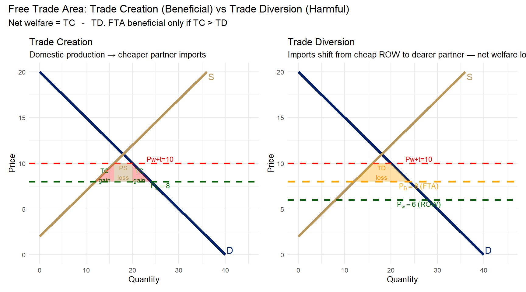
# Setup: Country A imports good X.
# Partner B price PB = 8; Rest-of-World price Pw = 6; MFN tariff t = 4.
# Domestic supply Qs = 2P - 4; Domestic demand Qd = 40 - 2P.
# Pre-FTA (Pw+t=10): Qs=16, Qd=20, M=4.
# Post-FTA with B (PB=8): Qs=12, Qd=24, M=12.

p1 <- ggplot() +
  geom_segment(aes(x = 0, y = 20, xend = 40, yend =  0),
               colour = "#012169", linewidth = 1.5) +
  geom_segment(aes(x = 0, y =  2, xend = 36, yend = 20),
               colour = "#B9975B", linewidth = 1.5) +
  geom_hline(yintercept = 10, colour = "red",       linetype = "dashed", linewidth = 1) +
  geom_hline(yintercept =  8, colour = "darkgreen", linetype = "dashed", linewidth = 1) +
  annotate("polygon", x = c(16, 20, 20, 16), y = c(8, 8, 10, 10),
           fill = "#B9975B", alpha = 0.4) +
  annotate("polygon", x = c(20, 24, 20),     y = c(8, 8, 10),
           fill = "red",    alpha = 0.3) +
  annotate("polygon", x = c(16, 12, 16),     y = c(10, 8, 8),
           fill = "red",    alpha = 0.3) +
  annotate("text", x = 18,   y = 9.0,  label = "PS\nloss",  size = 2.8, colour = "#B9975B") +
  annotate("text", x = 21.5, y = 8.7,  label = "TC\ngain",  size = 2.8, colour = "darkgreen") +
  annotate("text", x = 14,   y = 8.7,  label = "TC\ngain",  size = 2.8, colour = "darkgreen") +
  annotate("text", x = 41,   y = 0.5,  label = "D",         size = 4,   colour = "#012169") +
  annotate("text", x = 37,   y = 19.5, label = "S",         size = 4,   colour = "#B9975B") +
  annotate("text", x = 26,   y = 10.5, label = "Pw+t=10",   size = 3,   colour = "red") +
  annotate("text", x = 26,   y =  7.5, label = "P[B]==8",   size = 3,   colour = "darkgreen", parse = TRUE) +
  labs(title    = "Trade Creation",
       subtitle = "Domestic production → cheaper partner imports",
       x = "Quantity", y = "Price") +
  scale_x_continuous(limits = c(0, 45)) +
  theme_minimal(base_size = 10)

p2 <- ggplot() +
  geom_segment(aes(x = 0, y = 20, xend = 40, yend =  0),
               colour = "#012169", linewidth = 1.5) +
  geom_segment(aes(x = 0, y =  2, xend = 36, yend = 20),
               colour = "#B9975B", linewidth = 1.5) +
  geom_hline(yintercept = 10, colour = "red",       linetype = "dashed", linewidth = 1) +
  geom_hline(yintercept =  8, colour = "orange",    linetype = "dashed", linewidth = 1.2) +
  geom_hline(yintercept =  6, colour = "darkgreen", linetype = "dashed", linewidth = 1) +
  annotate("polygon",
           x = c(12, 16, 20, 24, 12),
           y = c( 8, 10, 10,  8,  8),
           fill = "orange", alpha = 0.35) +
  annotate("text", x = 18,   y =  9.0, label = "TD\nloss",      size = 2.8, colour = "darkorange") +
  annotate("text", x = 26,   y = 10.5, label = "Pw+t=10",       size = 3,   colour = "red") +
  annotate("text", x = 26,   y =  7.5, label = "P[B]==8~(FTA)", size = 3,   colour = "orange",    parse = TRUE) +
  annotate("text", x = 26,   y =  5.5, label = "P[w]==6~(ROW)", size = 3,   colour = "darkgreen", parse = TRUE) +
  annotate("text", x = 41,   y =  0.5, label = "D",             size = 4,   colour = "#012169") +
  annotate("text", x = 37,   y = 19.5, label = "S",             size = 4,   colour = "#B9975B") +
  labs(title    = "Trade Diversion",
       subtitle = "Imports shift from cheap ROW to dearer partner — net welfare loss",
       x = "Quantity", y = "Price") +
  scale_x_continuous(limits = c(0, 45)) +
  theme_minimal(base_size = 10)

p1 + p2 +
  plot_annotation(
    title    = "Free Trade Area: Trade Creation (Beneficial) vs Trade Diversion (Harmful)",
    subtitle = expression(paste("Net welfare = TC ", phantom(x), "-", phantom(x), " TD. FTA beneficial only if TC > TD"))
  )

Figure 4: FTA: Trade Creation (gain, left) vs Trade Diversion (loss, right) Source: Author’s illustration.

Current FTA Negotiations: Key Issues (I)

India-UK FTA (under negotiation, 2025):

  • UK wants: lower Indian tariffs on Scotch whisky, luxury cars, financial services
  • India wants: UK visa liberalization for IT professionals; lower tariffs on textiles, garments, processed food
  • Agricultural sticking points: UK dairy access, Indian basmati rice in UK market

India-EU FTA (restarted 2022):

  • EU demands: dairy market access, geographical indications (GI) protection, SPS harmonization
  • India demands: visa liberalization, textile market access
  • Agricultural sticking points: EU dairy (France, Netherlands), EU wines, Indian mango and rice exports

Trade Policy Instruments: A Quick Map

How Countries Restrict Trade (Preview for Lecture 7)

Tariff instruments: Basic customs duty (BCD); countervailing duty (CVD); anti-dumping duty (ADD); safeguard duty (temporary)

Non-tariff barriers: Quantitative restrictions (quotas); sanitary and phytosanitary (SPS) measures; technical barriers to trade (TBT); export subsidies (Amber Box, Blue Box under WTO)

India’s agricultural policy toolkit: Export restrictions (MEP, export bans); import restrictions (high tariffs, SPS barriers, MRL standards); domestic support (MSP, PM-KISAN, fertilizer subsidy); trade facilitation (APEDA market development, GI tags)

Next lecture (Lecture 7): Tariffs and quotas in detail — their welfare effects, WTO disciplines, and India’s use of these instruments.

Summary (I)

Lecture 6 — Core Concepts

  1. Terms of Trade — the export-import price ratio; India’s agricultural ToT is volatile and structurally challenged

  2. Prebisch-Singer Hypothesis — primary commodity prices decline relative to manufactures over the long run; India must move toward value-added exports

  3. Free trade — maximizes aggregate welfare through comparative advantage, but has distributional consequences; agriculture requires special treatment

  4. FTAs — second-best instruments driven by political economy; trade creation vs. diversion is the welfare test

Summary (II)

Lecture 6 — Core Concepts (continued)

  1. India’s FTA strategy — defensive on agriculture; offensive on services and labour-intensive manufactures; RCEP exit reflects agricultural protection priorities

  2. India-UAE CEPA — India’s new template: FTAs with non-agricultural partners are easier to conclude

  3. Key negotiating constraint — Agricultural market access is the binding constraint in all India’s major FTA negotiations

Next Lecture: Protectionism — Tariffs and Quotas

Lecture 7 — June 9, 2026

Instruments of Agricultural Protectionism:

  1. Tariffs — specific vs. ad valorem; partial and general equilibrium effects; welfare analysis (consumer surplus, producer surplus, government revenue)
  2. Quotas — tariff-rate quotas (TRQs) in WTO; welfare effects; rent seeking
  3. India’s tariff structure in agriculture — bound vs. applied tariffs; tariff water
  4. Non-tariff barriers — SPS standards, MRL limits, labelling requirements as instruments of protection
  5. India’s edible oil import protection story — a case study in the political economy of agricultural tariffs

Preparation: Review WTO’s Agricultural Agreement (Articles 4–6 on market access) and India’s Schedule of Concessions.

Appendix

Additional Resources

Further Reading

  • International Economics — Salvatore (Ch. 7-8)
  • International Economics — Appleyard & Field (Ch. 7-8)
  • RBI/DGCI&S/APEDA databases for latest data

Key Data Sources

  • DGCI&S: India’s merchandise trade
  • RBI: Balance of payments data
  • APEDA: Agricultural export statistics
  • WTO: Tariff and trade databases