Lecture 4: Theories of Trade II — Comparative Advantage

Econ 2203 | International Trade and Policy in Agriculture

Nithin M

Department of Development Economics

2026-05-16

Recap: The Gap in Smith’s Theory

Last lecture: Adam Smith argued that countries should export goods they produce absolutely more efficiently.

But this raises an obvious question:

What if one country is better at producing everything?

• Should the more efficient country trade at all?
• Should the less efficient country simply import everything?
• Would the inefficient country have any exports?

Smith’s absolute advantage gives no answer.

Stylised fact: The United States is more productive than Bangladesh in both textiles and aircraft. Yet the US imports textiles from Bangladesh. Why? → Enter David Ricardo (1817).

Ricardo’s Insight: What Matters is Relative Cost

Ricardo’s key insight was deceptively simple:

A country should specialise in the good for which it has the lower opportunity cost — regardless of absolute productivity.

Opportunity cost = what you must give up to produce one more unit of a good.

Even a country that is absolutely less efficient in everything can still gain from trade by exporting the good in which it is relatively less inefficient.

Analogy: A lawyer who types faster than her secretary still benefits from hiring the secretary — because the lawyer’s time is more valuably spent on legal work. The same logic applies to nations.

The Labor-Value Model: Notation

We work with the simplest possible model:

• Two countries: India (\(I\)) and the World (\(W\))
• Two goods: Rice (\(R\)) and Wheat (\(Wh\))
• One factor of production: Labour (\(L\))
• Technology: constant labour requirements per unit of output

Labour coefficients (units of labour per unit of output):

	Rice	Wheat
India	\(a_{LR}^{I}\)	\(a_{LWh}^{I}\)
World	\(a_{LR}^{W}\)	\(a_{LWh}^{W}\)

\(a_{LR}^{I}\) = labour hours required to produce one unit of Rice in India.

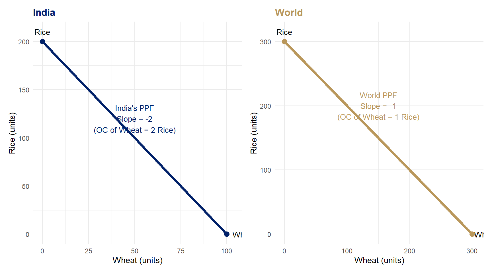
Numerical Example

Assume: each country has \(L = 600\) worker-hours. Labour required to produce one unit of output:

Country	Rice	Wheat
India	3 hours	6 hours
World	2 hours	2 hours

Labour coefficients: \(a_{LR}^{I} = 3\), \(a_{LWh}^{I} = 6\); \(a_{LR}^{W} = 2\), \(a_{LWh}^{W} = 2\). The World has absolute advantage in both goods (fewer hours needed per unit).

Opportunity costs:

\[OC_R^{I} = \frac{a_{LR}^{I}}{a_{LWh}^{I}} = \frac{3}{6} = \frac{1}{2} \text{ Wheat} \qquad OC_R^{W} = \frac{a_{LR}^{W}}{a_{LWh}^{W}} = \frac{2}{2} = 1 \text{ Wheat}\]

Comparison: \(OC_R^{I} = \tfrac{1}{2} < OC_R^{W} = 1\) \(\Rightarrow\) India has comparative advantage in Rice.

The Comparative Advantage Condition

Formal statement:

India has a comparative advantage in Rice if and only if:

\[\frac{a_{LR}^{I}}{a_{LWh}^{I}} < \frac{a_{LR}^{W}}{a_{LWh}^{W}}\]

Equivalently, rearranging:

\[\frac{a_{LR}^{I}}{a_{LR}^{W}} < \frac{a_{LWh}^{I}}{a_{LWh}^{W}}\]

India is relatively more efficient in Rice than in Wheat.

Key takeaway

Absolute productivity levels (\(a_{LR}^{I}\) vs \(a_{LR}^{W}\)) do not determine trade patterns. Relative productivity — the ratio of ratios — does.

Production Possibility Frontiers

With \(L = 600\) worker-hours, each country’s PPF is a straight line (constant opportunity cost):

India: \[3R + 6Wh = 600 \;\Rightarrow\; R + 2Wh = 200\] Slope \(= -2\) (give up 2 Rice per Wheat)

World: \[2R + 2Wh = 600 \;\Rightarrow\; R + Wh = 300\] Slope \(= -1\) (give up 1 Rice per Wheat)

The slope of the PPF = opportunity cost of Wheat.

library(ggplot2)
library(patchwork)

p1 <- ggplot() +
  geom_segment(aes(x=0, y=200, xend=100, yend=0),
               color="#012169", linewidth=1.5) +
  geom_point(aes(x=0, y=200), color="#012169", size=3) +
  geom_point(aes(x=100, y=0), color="#012169", size=3) +
  annotate("text", x=50, y=120,
           label="India's PPF\nSlope = -2\n(OC of Wheat = 2 Rice)",
           color="#012169", size=3.5, hjust=0.5) +
  annotate("text", x=103, y=0, label="Wheat", size=3.5, hjust=0) +
  annotate("text", x=0, y=210, label="Rice", size=3.5, hjust=0.5) +
  labs(title="India", x="Wheat (units)", y="Rice (units)") +
  theme_minimal(base_size=11) +
  theme(plot.title=element_text(color="#012169", face="bold"))

p2 <- ggplot() +
  geom_segment(aes(x=0, y=300, xend=300, yend=0),
               color="#B9975B", linewidth=1.5) +
  geom_point(aes(x=0, y=300), color="#B9975B", size=3) +
  geom_point(aes(x=300, y=0), color="#B9975B", size=3) +
  annotate("text", x=150, y=200,
           label="World PPF\nSlope = -1\n(OC of Wheat = 1 Rice)",
           color="#B9975B", size=3.5, hjust=0.5) +
  annotate("text", x=303, y=0, label="Wheat", size=3.5, hjust=0) +
  annotate("text", x=0, y=315, label="Rice", size=3.5, hjust=0.5) +
  labs(title="World", x="Wheat (units)", y="Rice (units)") +
  theme_minimal(base_size=11) +
  theme(plot.title=element_text(color="#B9975B", face="bold"))

p1 + p2

Figure 1: Production Possibility Frontiers: India and World Source: Author’s illustration.

The Terms of Trade Range

For trade to be mutually beneficial, the world price ratio must lie between the two autarky opportunity costs.

Autarky opportunity costs of Wheat (in terms of Rice):

\[OC_{Wh}^{I} = 2 \text{ Rice} \qquad OC_{Wh}^{W} = 1 \text{ Rice}\]

The terms of trade (price of Wheat relative to Rice) must satisfy:

\[1 < \frac{P_{Wh}}{P_R} < 2\]

• If \(P_{Wh}/P_R \leq 1\): India would not import Wheat (cheaper to produce at home)
• If \(P_{Wh}/P_R \geq 2\): World would not export Wheat (too expensive)
• At any intermediate price, both countries benefit.

Equilibrium ToT is determined by relative demand — say \(P_{Wh}/P_R = 1.5\).

Gains from Trade: India’s Perspective

Mechanism:

1. India fully specialises in Rice → produces (0 Wheat, 200 Rice)
2. Trades Rice for Wheat at world price \(P_{Wh}/P_R = 1.5\)
3. Consumption moves to a point above the PPF

The trade possibilities line starts at full specialisation (0, 200) with slope \(= -1.5\) (less steep in absolute value than the PPF slope \(-2\)).

Consumption bundle above the PPF = welfare gain!

library(ggplot2)

wheat_seq <- seq(0, 120, by=0.5)
rice_ppf   <- pmax(0, 200 - 2*wheat_seq)
rice_trade <- pmax(0, 200 - 1.5*wheat_seq)   # P_Wh/P_R = 1.5

df_ppf <- data.frame(wheat=wheat_seq, rice_ppf=rice_ppf, rice_trade=rice_trade)

ggplot(df_ppf, aes(x=wheat)) +
  geom_line(aes(y=rice_ppf), color="#012169", linewidth=1.5) +
  geom_line(aes(y=rice_trade), color="#B9975B", linewidth=1.5, linetype="dashed") +
  geom_point(aes(x=50, y=100), color="#012169", size=4) +
  annotate("text", x=54, y=100,
           label="Pre-trade\n(50Wh, 100R)", hjust=0, size=3.2, color="#012169") +
  geom_point(aes(x=67, y=100), color="#B9975B", size=4) +
  annotate("text", x=71, y=100,
           label="Post-trade\n(67Wh, 100R)\nabove PPF!",
           hjust=0, size=3.2, color="#B9975B") +
  geom_point(aes(x=0, y=200), color="darkgreen", size=3) +
  annotate("text", x=4, y=204,
           label="Full specialisation\n(0Wh, 200R)", hjust=0, size=3.2, color="darkgreen") +
  annotate("segment", x=50, y=100, xend=66, yend=100,
           arrow=arrow(length=unit(0.25,"cm")), color="darkgreen", linewidth=1) +
  annotate("text", x=55, y=108, label="Gains from trade!",
           color="darkgreen", size=3.5, fontface="bold") +
  labs(title="India specialises in Rice, trades for Wheat",
       subtitle="Trade line lies above the PPF — consumption set expands",
       x="Wheat (units)", y="Rice (units)") +
  scale_x_continuous(limits=c(0,120)) +
  scale_y_continuous(limits=c(0,220)) +
  theme_minimal(base_size=11)

Figure 2: India: Gains from Trade — Consuming Beyond the PPF Source: Author’s illustration.

Quantifying the Gains

Before trade (autarky): India produces and consumes on the PPF at \((Wh, R) = (50, 100)\)

After trade (at \(P_{Wh}/P_R = 1.5\)): India fully specialises → 200 Rice, trades \(\approx 100\) Rice for \(\approx 67\) Wheat: \[(Wh, R) \approx (67, 100)\]

Welfare gain: 17 more units of Wheat at the same Rice — the real wage of Indian workers rises.

The algebra: budget constraint under trade: \(R + 1.5 \cdot Wh = 200\)

Compare with autarky constraint: \(R + 2 \cdot Wh = 200\)

The trade budget line is flatter → larger feasible consumption set.

Consumer Preferences and Equilibrium

To find the exact equilibrium consumption bundle, we need indifference curves (ICs).

Properties of ICs:

• Downward sloping (MRS > 0)
• Convex to origin (diminishing MRS)
• Higher IC = higher utility

Autarky equilibrium (E1):

\[\text{MRS} = \frac{P_{Wh}}{P_R} = \frac{a_{LWh}^I}{a_{LR}^I} = 2\]

IC1 is tangent to the PPF at E1.

Free-trade equilibrium (E2):

IC2 is tangent to the trade possibilities line at E2.

Since IC2 is above IC1: trade raises welfare.

library(ggplot2)

wheat_seq <- seq(1, 105, by=0.5)
rice_ppf   <- pmax(0, 200 - 2*wheat_seq)
rice_trade <- pmax(0, 200 - 1.5*wheat_seq)   # P_Wh/P_R = 1.5 (was slope -1 — fixed)
rice_ic1   <- 5000 / wheat_seq               # U = sqrt(Wh*R), U1^2 = 50*100 = 5000
rice_ic2   <- 6700 / wheat_seq               # U2^2 = 67*100 = 6700 (E2 = (67,100) on IC2 & trade line)

df <- data.frame(
  wheat = wheat_seq,
  rice_ppf   = rice_ppf,
  rice_trade = rice_trade,
  rice_ic1   = rice_ic1,
  rice_ic2   = rice_ic2
)

ggplot(df, aes(x=wheat)) +
  geom_line(aes(y=rice_ppf,   color="PPF"),                   linewidth=1.5) +
  geom_line(aes(y=rice_trade, color="Trade Line"),             linewidth=1.5, linetype="dashed") +
  geom_line(aes(y=rice_ic1,   color="IC1 (autarky)"),          linewidth=1,   linetype="dotted") +
  geom_line(aes(y=rice_ic2,   color="IC2 (free trade)"),       linewidth=1,   linetype="dotted") +
  geom_point(aes(x=50,  y=100), color="#012169", size=3.5) +
  geom_point(aes(x=67,  y=100), color="#B9975B", size=3.5) +
  annotate("text", x=41, y=97,  label="E1\n(autarky)",   size=3, hjust=0) +
  annotate("text", x=69, y=106, label="E2\n(free trade)", size=3, hjust=0) +
  scale_color_manual(values=c(
    "PPF"             = "#012169",
    "Trade Line"      = "#B9975B",
    "IC1 (autarky)"   = "grey50",
    "IC2 (free trade)"= "darkgreen"
  )) +
  scale_y_continuous(limits=c(0, 250)) +
  scale_x_continuous(limits=c(0, 105)) +
  labs(title="Trade allows India to reach higher IC (IC2 > IC1)",
       x="Wheat", y="Rice", color="") +
  theme_minimal(base_size=11) +
  theme(legend.position="bottom")

Figure 3: Free Trade Equilibrium: IC tangent to Trade Possibilities Line Source: Author’s illustration.

Utility Maximisation Under Trade

Formal optimisation:

India maximises \(U(R, Wh)\) subject to the trade budget constraint:

\[\max_{R,\, Wh} \; U(R, Wh) \quad \text{s.t.} \quad P_R \cdot R + P_{Wh} \cdot Wh = P_R \cdot \bar{R}\]

where \(\bar{R} = 200\) (full specialisation output).

First-order condition:

\[\frac{MU_R}{MU_{Wh}} = \frac{P_R}{P_{Wh}} = \frac{1}{1.5}\]

Separation of production and consumption decisions:

Under free trade, India:

1. Produces where \(\text{slope of PPF} = P_R/P_{Wh}\) → full specialisation in Rice
2. Consumes where \(\text{MRS} = P_R/P_{Wh}\) → tangency of IC with trade line

These two points generally differ — the gap is filled by trade flows.

Key Assumptions of the Ricardian Model

Assumption	Implication
One factor (labour)	Ignores capital, land
Constant returns to scale	PPF is linear
Perfect factor mobility within country	Instantaneous reallocation
Immobile factors across countries	No international migration
No transport costs	TOT fully determines trade
Perfect competition	No strategic behaviour

Which matter most?

• Relaxing constant returns → curved PPF, partial specialisation
• Relaxing one factor → Heckscher-Ohlin model (Lecture 5)
• Adding transport costs → non-traded goods, border effects

The Ricardian Model: What It Gets Right

Remarkably robust predictions:

• Countries do specialise along lines of comparative advantage
• Trade raises real incomes on average
• Even the “least competitive” country has something to export
• Cannot explain intra-industry trade (→ new trade theory, Lecture 6)
• Extensions: Many goods (Dornbusch-Fischer-Samuelson chain); technology changes shift comparative advantage over time

Empirical support: Golub & Hsieh (2000) and Costinot et al. (2012) find strong evidence that labour productivity differences predict export patterns across countries. Predicts complete specialisation (rarely observed); says nothing about who within a country gains or loses.

Measuring Comparative Advantage: The Balassa Index

The Revealed Comparative Advantage (RCA) index (Balassa, 1965):

\[RCA_{ij} = \frac{X_{ij} / X_{i \cdot}}{X_{\cdot j} / X_{\cdot \cdot}}\]

where:

• \(X_{ij}\) = country \(i\)’s exports of good \(j\)
• \(X_{i\cdot}\) = country \(i\)’s total exports
• \(X_{\cdot j}\) = world exports of good \(j\)
• \(X_{\cdot\cdot}\) = world total exports

Interpretation:

• \(RCA_{ij} > 1\): country \(i\) has a comparative advantage in good \(j\)
• \(RCA_{ij} < 1\): country \(i\) has a comparative disadvantage in good \(j\)

India’s RCA in Agricultural Products

library(ggplot2)

rca_data <- data.frame(
  commodity = c("Spices", "Rice", "Oil Meals", "Cotton",
                "Marine\nProducts", "Fruits &\nVegetables",
                "Processed\nFood", "Edible Oil"),
  rca  = c(5.1, 4.8, 3.8, 3.2, 2.9, 1.4, 0.9, 0.3),
  type = c("Comp. Adv.", "Comp. Adv.", "Comp. Adv.", "Comp. Adv.",
           "Comp. Adv.", "Comp. Adv.", "No Adv.", "No Adv.")
)
rca_data$commodity <- factor(rca_data$commodity,
                              levels=rca_data$commodity[order(rca_data$rca)])

ggplot(rca_data, aes(x=commodity, y=rca, fill=type)) +
  geom_col(width=0.7) +
  geom_hline(yintercept=1, linetype="dashed", color="red", linewidth=0.8) +
  annotate("text", x=0.8, y=1.18, label="RCA = 1 (threshold)", color="red", size=3.5) +
  scale_fill_manual(values=c("Comp. Adv."="#012169", "No Adv."="#cccccc")) +
  coord_flip() +
  labs(title="India's Revealed Comparative Advantage (Balassa Index)",
       subtitle="RCA > 1 = comparative advantage; FY2024 DGCI&S data",
       x=NULL, y="RCA Index (Balassa)", fill=NULL) +
  theme_minimal(base_size=11) +
  theme(legend.position="bottom")

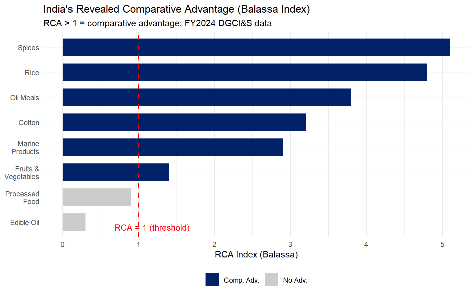
Figure 4: India: Revealed Comparative Advantage in Agricultural Products (FY2024) Source: Author’s calculations using DGCI&S / UN Comtrade data.

India: Rice as the Flagship Export

India’s Rice sector — Ricardo in practice:

• India is the world’s largest rice exporter (>22% of global exports, FY2024)
• Rice cultivation is labour-intensive — India’s abundant factor
• Relative labour productivity in rice > relative labour productivity in capital-intensive goods

Policy tension: September 2023: India imposed a 25% export duty on non-Basmati white rice → global rice prices spiked 15%.

\[P_R^{\text{world}} \uparrow \Rightarrow \text{India's ToT deteriorate for future exporters}\]

The ban is welfare-reducing under comparative advantage theory: India surrenders gains from trade to achieve food security goals. Central tension: Static efficiency ↔︎ food security; comparative advantage ↔︎ strategic reserves; export competitiveness ↔︎ domestic price stability.

Comparative Advantage: Summary

Core results of the Ricardian Model:

1. Trade is driven by relative, not absolute, productivity differences
2. Comparative advantage condition: \(\frac{a_{LR}^{I}}{a_{LWh}^{I}} < \frac{a_{LR}^{W}}{a_{LWh}^{W}}\)
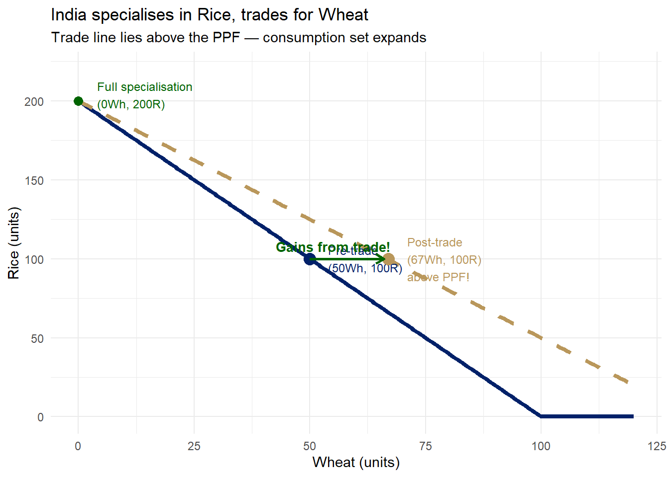
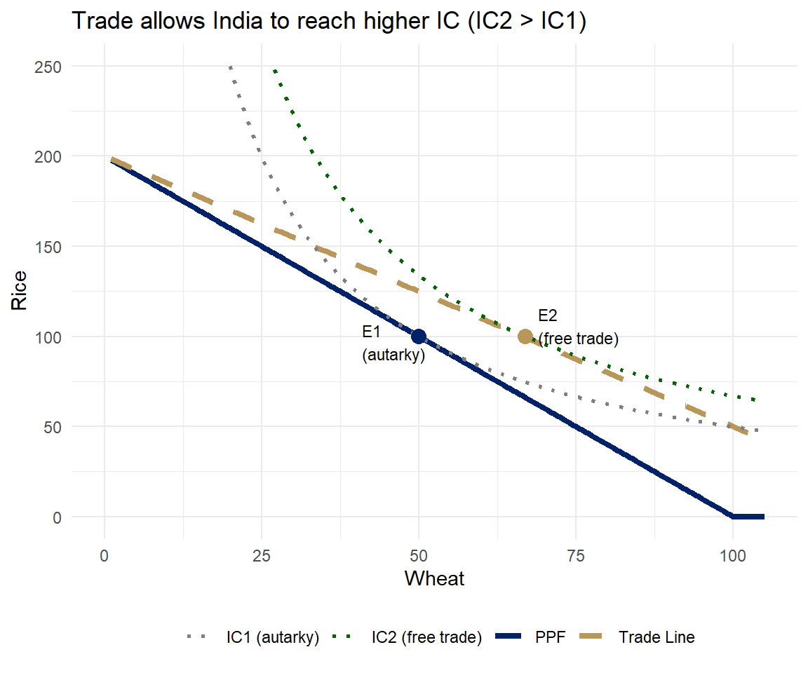
3. Gains from trade: consumption bundle moves beyond the PPF
4. Terms of trade must lie between autarky opportunity costs: \(OC_R^W < \frac{P_R}{P_{Wh}} < OC_R^I\)
5. Both countries gain — even the absolutely less productive one

Empirical verdict: Labour productivity differences strongly predict export patterns — Costinot et al. (2012) find R² ≈ 0.9 across countries. India’s rice exports (RCA = 4.8) confirm comparative advantage. Complete specialisation is rarely observed in practice, and short-run distributional losses are documented — but aggregate welfare gains are robust.

What Ricardo cannot explain: Why labour productivity differs (→ H-O model); income distribution effects (→ Stolper-Samuelson); intra-industry trade (→ Lecture 6)

Appendix

Additional Resources

Further Reading

• International Economics — Salvatore (Ch. 3)
• International Economics — Appleyard & Field (Ch. 3)
• RBI/DGCI&S/APEDA databases for latest data

Key Data Sources

• DGCI&S: India’s merchandise trade
• RBI: Balance of payments data
  
• APEDA: Agricultural export statistics
• WTO: Tariff and trade databases