Lecture 3: Theories of International Trade I

Econ 2203 | International Trade and Policy in Agriculture

Nithin M

Department of Development Economics

2026-05-09

The Central Question

Why do countries trade?

This question has occupied economists for over 500 years. Three broad answers have emerged:

1. Mercantilism (1500–1750): Trade is a zero-sum competition for power; exports = good, imports = bad; accumulate gold

2. Absolute Advantage — Adam Smith (1776): Trade is win-win; each country specialises in what it produces most efficiently

3. Comparative Advantage — David Ricardo (1817): Even if one country is better at everything, both countries gain from trade based on relative costs

Why theory matters for policy: India bans rice exports → mercantilist instinct. India signs FTAs → comparative advantage logic. These theories are the intellectual foundation of every trade policy debate happening right now.

Trade theory timeline (I): early foundations

• Mercantilism (1500–1750): wealth = gold; maximise trade surplus
• Smith (1776): absolute advantage (higher productivity)
• Ricardo (1817): comparative advantage (lower opportunity cost)
• H–O (1933): trade reflects factor endowments
• Big shift: from “win–lose trade” → gains from specialization

Trade theory timeline (II): modern extensions

• Leontief (1953): data challenge to simple H–O predictions
• Krugman (1970s–80s): scale economies + imperfect competition
• Porter (1990s): national competitiveness and institutions
• Melitz (2000s): firm heterogeneity; only productive firms export
• Course roadmap: by Lecture 6 we cover the arc; today starts with mercantilism + Smith

Mercantilism: the setting

• Dominant European doctrine: 1500–1750
• Bullion money: gold/silver treated as “wealth”
• Nation-states + colonial expansion + chartered companies

Mercantilism: core beliefs

• Wealth ≈ gold/silver stock
• Goal: export > import (surplus)
• Trade seen as zero-sum
• State actively manages trade (tariffs, subsidies, monopolies)

Modern echo: “increase the trade surplus” rhetoric often reflects mercantilist instincts.

Mercantilist policies (export side)

• Export subsidies / rebates to push exports
• Chartered trading companies (EIC, VOC) with monopoly rights
• Shipping restrictions (Navigation Acts) to control trade routes

Mercantilist policies (import side + currency)

• Import duties / quotas to restrict imports
• State monopolies to control strategic goods
• Currency undervaluation to make exports cheaper

Modern equivalents (examples)

• Export rebates: RoDTEP (India)
• Import duties: India’s tariff schedule
• Trading houses: MMTC/STC (public trading)
• Undervaluation episode: China (2000s)

Mercantilism isn’t always “irrational”; the error is the zero-sum worldview.

Colonial trade: British mercantilism in India

• India as raw material source + captive market
• Cotton chain: India → Manchester mills → textiles back to India
• Trade rules tilted toward Britain (favouring British textiles)

The “drain” idea (why this matters)

• Naoroji: colonial trade + administration created a systematic transfer outward
• Channels: home charges, interest payments, profits remitted
• Big estimates exist (e.g., Patnaik 2018 ≈ $45T PV) — methodology debated

Agricultural dimension

• Cash-crop push (indigo/opium/jute) could displace food crops
• Higher food vulnerability + famine risk (Bengal 1943)
• Key point: institutions + trade policy shape what gets produced

The Drain of Wealth: Naoroji’s Evidence

Dadabhai Naoroji’s Drain Theory

• Naoroji (1901): Poverty and Un-British Rule in India
• Calculated that Britain extracted £200–300 million per year from India as “drain”
• Home charges: India paid for British administration costs, interest on British-held debt, railway profits
• The mechanism: India exported goods but received paper IOUs rather than gold — a systematic wealth transfer disguised as trade

“England has impoverished India by her own prosperity.” — Dadabhai Naoroji, 1901

Modern reassessment: Economists Utsa Patnaik (2018) and Sashi Tharoor (Inglorious Empire, 2017) updated Naoroji’s estimates. The drain theory remains contested on methodology but its directional conclusion — that colonial trade systematically transferred wealth from India to Britain — is broadly accepted.

Critique of Mercantilism

David Hume’s price-specie-flow mechanism (1752)

Mercantilism has a self-defeating logic:

1. Country A runs a trade surplus → gold flows in → money supply rises
2. More money → prices rise (quantity theory of money: MV = PQ)
3. Higher prices → Country A’s exports become more expensive
4. Exports fall, imports rise → trade surplus disappears automatically

Adam Smith’s critique (1776): “Wealth of a nation is not measured by the gold in its vaults but by the goods and services it can produce and consume”; import restrictions reduce consumption possibilities

The fundamental error: Mercantilists confused the means (gold) with the end (well-being). A country with more gold but fewer goods is poorer, not richer.

Modern parallel: Japan in the 1980s ran huge trade surpluses with the USA. Was Japan richer for it? Its citizens had high savings but lower consumption than Americans with similar incomes — a classic mercantilist outcome.

Mercantilist Arithmetic: Why the Logic Fails

The mercantilist objective function

A nation seeks to accumulate gold \(G\) by maximising its trade surplus:

\[\text{Objective: } \max\; G = X - M\]

\[\Rightarrow \text{policy prescriptions: } X \uparrow \text{ (export subsidies)}, \quad M \downarrow \text{ (tariffs, prohibitions, bans)}\]

The zero-sum fallacy: If all \(N\) nations simultaneously pursue a surplus:

\[\sum_{i=1}^{N}(X_i - M_i) = 0 \quad \forall \text{ nations simultaneously}\]

Hume’s price-specie-flow refutation (1752): Even a single nation’s surplus is self-correcting:

\[\text{Gold inflow} \;\Rightarrow\; M_s \uparrow \;\Rightarrow\; P \uparrow \;\Rightarrow\; X \downarrow,\; M \uparrow \;\Rightarrow\; \text{surplus eliminated}\]

A mercantilist surplus is self-defeating: the very gold inflow it generates raises domestic prices, eroding the export competitiveness that created the surplus.

Smith’s Critique: Real Wealth vs Gold

Smith’s fundamental restatement

Mercantilists measured national wealth by the gold stock. Smith showed the correct measure is real consumption:

\[W_{\text{real}} = \frac{\text{goods and services consumed}}{P} \;\neq\; \text{gold stock}\]

The trade restriction paradox — applied to India

If India bans rice exports to keep supply at home: \[W_{\text{domestic,rice}} \uparrow \quad \text{(rice cheaper domestically)}\] \[W_{\text{global}} = 0 \quad \text{(no new rice created — redistributed, not added)}\]

If instead India exports rice and specialises: \[W_{\text{global}} \uparrow \quad \text{(specialisation gains; world output expands)}\] \[W_{\text{India}} \uparrow \quad \text{(farmers earn more; import cheaper goods)}\]

“It is the maxim of every prudent master of a family, never to attempt to make at home what it will cost him more to make than to buy.” — Wealth of Nations, Book IV, Ch. 2

National self-sufficiency achieved through restriction destroys, not creates, real wealth.

Mercantilism vs Smith: Policy Implications

Dimension	Mercantilism	Adam Smith
Goal	National power / gold accumulation	National prosperity / consumption
View of trade	Zero-sum: one nation’s gain = another’s loss	Positive-sum: specialisation grows world output
Role of imports	Evil — gold drains out	Beneficial — access to cheaper goods
Role of exports	Good — gold flows in	A means to pay for imports
State role	Regulate all trade; grant monopolies	Laissez-faire; let markets direct resources
India example (2023)	Rice/wheat export ban — hoard grain, protect prices	RCEP/FTA participation — specialise, exchange

The modern policy echo: Every time an Indian policymaker imposes an export ban to protect domestic consumers, they invoke mercantilist logic. Every time an economist argues for free trade to raise farmer incomes, they invoke Smith. Both impulses co-exist in India’s agricultural trade policy — understanding the theory clarifies which logic applies when.

Neo-Mercantilism: Export-Led Development Strategies

Modern mercantilist practices

• Export-led growth strategy (China, South Korea, Germany): Use undervalued currency and export subsidies to drive export surplus; accumulate foreign exchange reserves
• Currency undervaluation: China’s renminbi was widely believed to be 20–40% undervalued vs USD in 2000s
• “Beggar-thy-neighbour” policies: Competitive devaluations — my currency devaluation boosts my exports at your expense
• Industrial policy for export champions: China’s $5 trillion in state subsidies to EVs, solar panels (WTO disputes pending)
• India’s FTP 2023–28 target of $2 trillion exports has a mercantilist flavour — emphasises export growth

The “China is mercantilist” debate: China kept RMB undervalued by ~20–40%, providing massive subsidies to export industries → $3T+ in foreign exchange reserves. Critics: unfair competition. China’s response: infant industry protection, just like US and UK in 19th century. Who is right? Both, somewhat.

Neo-Mercantilism: Critique and Assessment

Critical Analysis of Neo-Mercantilist Strategies

While export-led growth produced remarkable results in East Asia (South Korea, Taiwan, China), neo-mercantilism has fundamental limitations:

• Not universally replicable: If all developing countries simultaneously pursue export surpluses, not all can succeed — the global sum of surpluses must be zero
• Trading partner retaliation: Persistent surpluses invite countervailing duties, anti-dumping actions, and trade wars (e.g., US-China trade war, 2018–present)
• Domestic welfare cost: Currency undervaluation raises the cost of imports for domestic consumers; workers in export industries may face poor conditions
• Bretton Woods system collapse (1971): The original system broke down partly because of mercantilist pressures from surplus countries

For India: The challenge is to use strategic export promotion (FTP, APEDA, SEZs) without triggering WTO violations or partner retaliation.

Adam Smith’s Insight

The context: Wealth of Nations (1776)

• Published the same year as the American Declaration of Independence
• A direct intellectual attack on mercantilism and the colonial trade system
• Argued for free markets and free trade as the sources of national wealth

“If a foreign country can supply us with a commodity cheaper than we ourselves can make it, better buy it of them with some part of the produce of our own industry, employed in a way in which we have some advantage.” — Adam Smith, Wealth of Nations, Book IV, Ch. 2

Smith’s core insight: Trade is not zero-sum — both countries gain. Each country should produce what it is best at — absolute advantage. The standard of living rises when countries specialise and exchange.

Absolute advantage: Country A has an absolute advantage in producing good X if it can produce more units of X per unit of labour than Country B.

Assumptions of the Absolute Advantage Model

Assumption	Implication
Two countries (A, B)	Tractable bilateral comparison
Two goods (X, Y)	One good per country’s advantage
One factor — labour	Productivity differences drive trade
Labour mobile within country	Workers shift between sectors freely
Labour immobile across countries	No international migration
Constant returns to scale	Linear PPF; constant opportunity costs
Perfect competition	Prices equal marginal (labour) costs
Full employment	All labour is always in use
No transport costs	World price fully determines trade

Key limitation: If one country is better at both goods, the model predicts no trade. Ricardo’s comparative advantage (Lecture 4) resolves this.

Absolute Advantage: Formal Definition

Setting up the model

Assumptions: two countries (A, B), two goods (X, Y), one factor (labour), labour mobile within but immobile between countries, constant returns to scale, full employment.

Country A has an absolute advantage in Good X if:

\[a_{LX}^A < a_{LX}^B\]

where \(a_{LX}\) = labour required to produce one unit of Good X.

Units of output per worker-day:

	Good X	Good Y
Country A	\(\frac{1}{a_{LX}^A}\)	\(\frac{1}{a_{LY}^A}\)
Country B	\(\frac{1}{a_{LX}^B}\)	\(\frac{1}{a_{LY}^B}\)

Country A has absolute advantage in X if the value in row A, column X exceeds the value in row B, column X.

Smith’s prescription: A has absolute advantage in X → A should export X. B has absolute advantage in Y → B should export Y. Both specialise → both gain.

Absolute Advantage: India vs USA (Salvatore Notation)

Production possibilities (units per worker-day)

Following Salvatore (2013, Ch. 2) — two nations, two commodities:

	India	USA
Rice (units/worker-day)	4	1
Wheat (units/worker-day)	1	3

• Rice: India produces 4 vs USA’s 1 → India has absolute advantage in Rice
• Wheat: USA produces 3 vs India’s 1 → USA has absolute advantage in Wheat

Opportunity costs (= PPF slopes):

\[\text{India: OC of 1 Wheat} = 4 \text{ Rice} \quad (\text{steep PPF — Rice-abundant})\] \[\text{USA: OC of 1 Wheat} = \tfrac{1}{3} \text{ Rice} \quad (\text{flat PPF — Wheat-efficient})\]

Each country has 40 worker-days of labour. PPF equations (linear = constant opportunity cost): \[\text{India: } R = 160 - 4W \qquad \text{USA: } R = 40 - \tfrac{1}{3}W\]

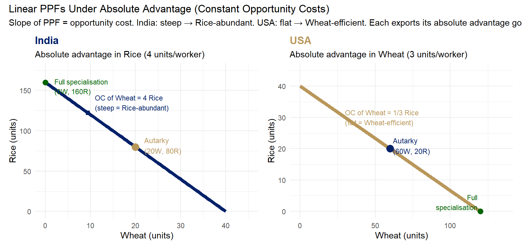
# India: L = 40 worker-days. Rice max = 40×4 = 160; Wheat max = 40×1 = 40
# PPF: R = 160 - 4W  (OC of 1 Wheat = 4 Rice → steep slope)
# USA: L = 40 worker-days. Rice max = 40×1 = 40; Wheat max = 40×3 = 120
# PPF: R = 40 - (1/3)W  (OC of 1 Wheat = 1/3 Rice → flat slope)

wheat_india <- seq(0, 40, by = 0.5)
rice_india  <- 160 - 4 * wheat_india

wheat_usa <- seq(0, 120, by = 0.5)
rice_usa  <- 40 - (1/3) * wheat_usa

p1 <- ggplot() +
  geom_line(data = data.frame(w = wheat_india, r = rice_india),
            aes(x = w, y = r), color = "#012169", linewidth = 2) +
  geom_point(aes(x = 20, y = 80), color = "#B9975B", size = 4) +
  annotate("text", x = 22, y = 82,
           label = "Autarky\n(20W, 80R)", size = 3.2, hjust = 0, color = "#B9975B") +
  geom_point(aes(x = 0, y = 160), color = "darkgreen", size = 3) +
  annotate("text", x = 2, y = 155,
           label = "Full specialisation\n(0W, 160R)", size = 3, hjust = 0, color = "darkgreen") +
  annotate("segment", x = 5, y = 140, xend = 10, yend = 120,
           arrow = arrow(length = unit(0.2, "cm")),
           color = "#012169", linewidth = 0.8) +
  annotate("text", x = 11, y = 135,
           label = "OC of Wheat = 4 Rice\n(steep = Rice-abundant)",
           size = 3, hjust = 0, color = "#012169") +
  labs(title    = "India",
       subtitle = "Absolute advantage in Rice (4 units/worker)",
       x = "Wheat (units)", y = "Rice (units)") +
  scale_x_continuous(limits = c(0, 45)) +
  scale_y_continuous(limits = c(0, 175)) +
  theme_minimal(base_size = 11) +
  theme(plot.title = element_text(color = "#012169", face = "bold", size = 13))

p2 <- ggplot() +
  geom_line(data = data.frame(w = wheat_usa, r = rice_usa),
            aes(x = w, y = r), color = "#B9975B", linewidth = 2) +
  geom_point(aes(x = 60, y = 20), color = "#012169", size = 4) +
  annotate("text", x = 62, y = 21,
           label = "Autarky\n(60W, 20R)", size = 3.2, hjust = 0, color = "#012169") +
  geom_point(aes(x = 120, y = 0), color = "darkgreen", size = 3) +
  annotate("text", x = 118, y = 3,
           label = "Full\nspecialisation", size = 3, hjust = 1, color = "darkgreen") +
  annotate("text", x = 30, y = 30,
           label = "OC of Wheat = 1/3 Rice\n(flat = Wheat-efficient)",
           size = 3, hjust = 0, color = "#B9975B") +
  labs(title    = "USA",
       subtitle = "Absolute advantage in Wheat (3 units/worker)",
       x = "Wheat (units)", y = "Rice (units)") +
  scale_x_continuous(limits = c(0, 135)) +
  scale_y_continuous(limits = c(0, 45)) +
  theme_minimal(base_size = 11) +
  theme(plot.title = element_text(color = "#B9975B", face = "bold", size = 13))

p1 + p2 + plot_annotation(
  title    = "Linear PPFs Under Absolute Advantage (Constant Opportunity Costs)",
  subtitle = "Slope of PPF = opportunity cost. India: steep → Rice-abundant. USA: flat → Wheat-efficient. Each exports its absolute advantage good."
)

Figure 1: Linear PPFs: India and USA — Absolute Advantage (constant opportunity costs) Source: Author’s illustration.

Gains from Trade: India and USA Under Absolute Advantage

Without trade — autarky (labour split 50/50)

	India	USA	World
Rice (units)	80	20	100
Wheat (units)	20	60	80

With trade — full specialisation

	India	USA	World
Rice (units)	160	0	160
Wheat (units)	0	120	120

World gains: \(\Delta \text{Rice} = +60 \text{ units}\) (+60%); \(\Delta \text{Wheat} = +40 \text{ units}\) (+50%)

At terms of trade 2 Rice = 1 Wheat (India exports Rice, imports Wheat): both countries consume outside their individual PPFs — trade expands the consumption frontier. Absolute advantage gives each nation a clear signal about where to specialise.

Numerical Example: India and Bangladesh

The production possibilities

Country	Rice (quintals/worker-day)	Jute (metres/worker-day)
India	4	2
Bangladesh	1	4

• Rice: India has absolute advantage. Jute: Bangladesh has absolute advantage.

Before trade (autarky — 50/50 split, 100 workers each):

Country	Rice	Jute
India	200	100
Bangladesh	50	200
World total	250	300

After full specialisation:

Country	Rice	Jute
India	400	0
Bangladesh	0	400
World total	400 (+60%)	400 (+33%)

Both countries consume more at terms of trade 1:1 — trade is genuinely win-win.

India’s Absolute Advantage in Agriculture

Where India has clear absolute advantage

Commodity	India’s global rank	Key advantage
Milk production	#1	230M+ cattle; Operation Flood legacy
Pulse production	#1	Dryland farming expertise; diverse varieties
Spice production	#1	Tropical climate; accumulated expertise
Rice production	#2 (after China)	Diverse agro-climates; Green Revolution

Why India has these advantages: Diverse agro-climatic zones (12 of 15 major global types); abundant agricultural labour (50% of workforce); long cultivation history → accumulated knowledge

Spices: India’s oldest absolute advantage. India produces ~75% of world’s spices; exports ~$3.7B in spices (FY2024). The same advantage that drove European colonial expansion to India’s coasts persists today — climate, soils, and accumulated expertise that competitors cannot easily replicate.

India’s Agricultural Productivity: Absolute Advantage Indicators

labour_prod <- data.frame(
  commodity   = c("Basmati Rice", "Non-Basmati\nRice", "Cotton", "Spices\n(Pepper)",
                  "Wheat", "Soybean", "Maize"),
  india_yield = c(3.8, 4.1, 2.1, 2.8, 3.5, 1.2, 3.0),
  world_yield = c(2.9, 4.4, 2.0, 1.5, 3.5, 2.8, 5.8),
  india_adv   = c(TRUE, FALSE, TRUE, TRUE, FALSE, FALSE, FALSE)
)

labour_prod <- labour_prod |>
  arrange(india_yield / world_yield) |>
  mutate(
    commodity = factor(commodity, levels = commodity),
    ratio     = round(india_yield / world_yield, 2)
  )

ggplot(labour_prod, aes(x = commodity, y = ratio, fill = india_adv)) +
  geom_col(width = 0.7) +
  geom_hline(yintercept = 1, linetype = "dashed", color = "red", linewidth = 1) +
  geom_text(aes(label = paste0(ratio, "x")), hjust = -0.1, size = 3.2) +
  annotate("text", x = 1, y = 1.1,
           label = "World average = 1.0", color = "red", size = 3.5) +
  scale_fill_manual(
    values = c("TRUE" = "#012169", "FALSE" = "#cccccc"),
    labels = c("TRUE" = "India's absolute advantage", "FALSE" = "Below world average")
  ) +
  coord_flip() +
  labs(
    title    = "India's Yield Productivity Relative to World Average",
    subtitle = "Above 1.0x = India produces more per hectare than world average (absolute advantage indicator)",
    x = NULL, y = "India Yield / World Average Yield", fill = NULL
  ) +
  scale_y_continuous(limits = c(0, 2.2)) +
  theme_minimal(base_size = 11) +
  theme(legend.position = "bottom")

Figure 2: India’s Yield Productivity Relative to World Average — Absolute Advantage Indicators Source: FAO, FAOSTAT (2023).

Reading the chart: Spices (Pepper) at 1.87x and Basmati Rice at 1.31x show the strongest absolute advantage — India produces far more per hectare than the world average. Maize (0.52x) and Soybean (0.43x) show India well below world average — not where export effort should be directed. Cotton (1.05x) and Non-Basmati Rice (0.93x) are near parity — other factors (price, quality, logistics) determine trade patterns.

Limitations of Absolute Advantage Theory

Theoretical limitations

1. Ignores the case where one country is better at everything — If India has absolute advantage in both rice and jute, Smith’s theory says Bangladesh should not trade → clearly wrong
2. Labour-only model — Ignores capital, land, technology; these matter enormously in agriculture
3. Constant returns to scale — Real agriculture has diminishing returns (limited fertile land)
4. Transport costs ignored — A commodity with a slight absolute advantage may not be worth trading if freight is high

Practical limitations

5. No room for trade policy — The model says free trade is always optimal; ignores infant industry, food security arguments
6. No product quality differences — India exports basmati rice (premium quality) and non-basmati (commodity); model treats all rice as identical
7. Static model — Absolute advantage can change over time (South Korea: no electronics advantage in 1960; now it does)

Full employment assumption: In reality, India has seasonal unemployment; trade may employ idle labour rather than divert it.

The Problem with Absolute Advantage

The critical case: What if one country is better at everything?

Suppose USA vs India:

Country	Wheat (tonnes/worker)	Software (units/worker)
USA	4	8
India	2	2

USA has absolute advantage in both wheat and software. Smith’s theory predicts: No basis for trade — India has no absolute advantage in anything.

But we know India and USA trade extensively! (India exports software services $80–100B/year + agricultural products)

What Smith missed — comparative advantage: Even though USA is better at both goods, the degree of advantage differs. USA is 2× better at wheat (4 vs 2) but 4× better at software (8 vs 2). USA has a stronger advantage in software → USA should specialise in software. India has a lesser disadvantage in wheat → India should specialise in wheat. This is comparative advantage — David Ricardo’s great insight. We prove this formally in Lecture 4.

Smith vs Mercantilism: A Summary Comparison

Dimension	Mercantilism	Adam Smith (Absolute Advantage)
Source of national wealth	Stock of gold and silver	Productive capacity; goods and services
Nature of trade	Zero-sum (one country’s gain = another’s loss)	Win-win (both countries gain from specialisation)
Objective of trade policy	Maximise exports; minimise imports	Maximise specialisation; allow free exchange
Role of government	Active: subsidise exports, restrict imports, grant monopolies	Minimal: allow markets to direct specialisation
Imports: good or bad?	Bad — gold flows out	Good — access to cheaper goods; frees resources for comparative advantage sectors
Trade balance	Surplus is the goal	Irrelevant; what matters is consumption possibilities
Colonies	Essential — raw material source + captive market	Unnecessary and harmful to the coloniser too (waste of resources)
Legacy	Colonial trade systems; modern currency wars	Foundation of free trade economics; WTO ideology

India Policy Application: Mercantilism vs Smith in Real Decisions

The rice export ban (2023): a case study

The mercantilist argument for the ban: - Domestic rice prices rising → risk food inflation rising → protect domestic consumers - Keep rice in India → ensure food security → classic mercantilist hoarding of “strategic resources”

The Smithian argument against the ban: - India has absolute (and comparative) advantage in rice → should be exporting, not restricting - Ban reduces income of 30 million paddy farmers; damages long-term export relationships

Who won? The ban was implemented in August 2023 — mercantilist/food security logic prevailed.

India’s trade policy oscillates between export restrictionism (rice ban, wheat ban, onion export bans) and export promotion (FTP 2023–28, APEDA support, RoDTEP). Both impulses co-exist because the political economy is complex: consumers want cheap food; farmers want high prices; government wants foreign exchange.

The Case of Indian Spices: Absolute Advantage in Action

India’s dominance in global spice markets

• Production: India produces 75% of world’s spices by volume; 50%+ by value
• Export performance (FY2024): $3.7 billion; 14% growth over FY2023

Spice	Export value	Top markets
Chilli	$982M	USA, Vietnam, Sri Lanka
Cumin	$700M	USA, Bangladesh, China
Cardamom	$350M	Saudi Arabia, UAE
Turmeric	$300M	Bangladesh, USA
Pepper	$190M	USA, Vietnam

Source of absolute advantage: Specific agro-climatic conditions (Kerala for pepper/cardamom, AP/Rajasthan for chilli/cumin) that cannot be replicated at comparable cost elsewhere

The search for direct sea routes to India’s spice markets was the primary driver of the “Age of Exploration” — Columbus was looking for a route to India’s spices when he accidentally reached the Americas. India’s spice export advantage today is the same: climate, soils, and accumulated expertise that competitors cannot easily replicate.

Summary: Mercantilism and Absolute Advantage

Key points from Lecture 3

Mercantilism (1500–1750): - Wealth = gold; goal = trade surplus; trade is zero-sum - Led to colonial exploitation, including India’s “drain of wealth” - Critiqued by Hume (price-specie-flow) and Smith (wealth is production, not gold)

Absolute Advantage (Adam Smith, 1776): - Each country should specialise in what it produces most efficiently - Trade is win-win — world production rises with specialisation

The fatal limitation: What if one country is better at everything? Smith cannot explain trade between USA and India. This is the gap Ricardo fills with comparative advantage.

• India and Bangladesh example: rice vs jute — both gain from specialisation under absolute advantage.

Key Takeaways: Lecture 3

What we covered today

• Mercantilism: Trade as power accumulation; maximise surplus; zero-sum worldview → systematically flawed, but echoes persist in modern policy
• Colonial trade in India: British mercantilism extracted surplus, destroyed Indian textile industry → “drain of wealth” (Naoroji)
• Hume and Smith’s critiques: Trade surpluses are self-correcting (price-specie-flow); real wealth is productive capacity, not gold
• Absolute advantage: Specialise in what you produce with highest absolute efficiency; trade is win-win
• Fundamental limitation: Absolute advantage cannot explain trade when one country is more efficient in everything → sets up Ricardo’s comparative advantage

• India’s absolute advantages: Rice, spices, pulses, milk, jute — rooted in agro-climatic endowments and accumulated human capital

Next Lecture: Lecture 4

Theories of International Trade II — Comparative Advantage (May 19, 2026)

We will cover:

• David Ricardo (1817): The most profound insight in economics — comparative advantage
• The opportunity cost logic: Why the relative cost, not absolute cost, determines trade patterns
• Formal model: Two countries, two goods, with full numerical derivation
• Production Possibility Frontier (PPF): Formal diagrammatic treatment
• Empirical evidence: Does the Ricardian model predict actual trade patterns?

Suggested reading

• Krugman, Obstfeld & Melitz, International Economics, Ch. 3
• Ricardo, D. (1817). Principles of Political Economy and Taxation, Ch. 7 (excerpt)
• Goldin, I. and Reinert, K. (2012). Globalization for Development, Ch. 2

Key question to prepare:

If India is only half as productive as the USA in all agricultural commodities, should India and USA trade at all? If yes, what should each produce?

Appendix

Additional Resources

Further Reading

• International Economics — Salvatore (Ch. 2-3)
• International Economics — Appleyard & Field (Ch. 2-3)
• RBI/DGCI&S/APEDA databases for latest data

Key Data Sources

• DGCI&S: India’s merchandise trade
• RBI: Balance of payments data
  
• APEDA: Agricultural export statistics
• WTO: Tariff and trade databases