Lecture 1: Introduction to International Trade

Econ 2203 | International Trade and Policy in Agriculture

Nithin M

Department of Development Economics

2026-04-25

Course Overview: Econ 2203

What this course is about

• The economics of trade between nations — with a focus on agricultural commodities
• Why countries trade, who gains, who loses, and what policy should do about it
• India’s position in global agricultural trade and key policy instruments

Learning objectives

• Master classical and modern theories of trade
• Analyse India’s agricultural trade flows and policy environment
• Evaluate trade policy tools: tariffs, quotas, subsidies, SPS measures
• Apply WTO frameworks to real agricultural trade disputes

Assessment: Mid-semester exam (30%) · End-semester exam (40%) · Term paper (20%) · Participation (10%)

Course Roadmap: Lectures 1–9

Lec	Topic	Date
1	Introduction to International Trade	Apr 28
2	Features & Internal vs International Trade	May 5
3	Theories I — Mercantilism & Absolute Advantage	May 12
4	Theories II — Comparative Advantage	May 19
5	Theories III — Factor Endowments (H-O Model)	May 26
6	New Trade Theory & Intra-Industry Trade	Jun 2
7	Terms of Trade & Trade Gains	Jun 9
8	Trade Policy: Tariffs	Jun 16
9	Trade Policy: Non-Tariff Barriers	Jun 23

Course Roadmap: Lectures 10–18

Lec	Topic	Date
10	Balance of Payments & Exchange Rates	Jun 30
11	WTO Framework & Agreements	Jul 7
12	Agreement on Agriculture (AoA)	Jul 14
13	SPS & TBT Measures in Agriculture	Jul 21
14	India’s Foreign Trade Policy	Jul 28
15	Regional Trade Agreements — ASEAN, SAFTA	Aug 4
16	Agricultural Price Policy & Trade	Aug 11
17	Food Security and Trade Nexus	Aug 18
18	Contemporary Issues & Revision	Aug 25

What is International Trade?

Definition

International trade is the cross-border exchange of goods, services, and capital between residents of different countries.

Three dimensions of trade

• Merchandise trade — physical goods: rice, wheat, machinery, petroleum
• Services trade — IT services, tourism, financial services, education
• Capital flows — foreign direct investment, portfolio investment, remittances

Why it matters for agricultural economists

• India earns ~₹3.6 lakh crore from agricultural exports annually
• Global price signals directly affect domestic farm prices
• WTO rules constrain domestic agricultural support policies

Core insight: Trade is fundamentally about countries doing what they are relatively better at, and exchanging the surplus — creating gains for all participants.

Why Do Nations Trade?

Supply-side reasons

• Resource endowments — India has fertile Indo-Gangetic plains; Brazil has Amazon basin → different agricultural outputs
• Technology differences — Netherlands uses precision horticulture; India relies on labour-intensive methods
• Specialization gains — Focusing on fewer products reduces unit cost
• Economies of scale — Large production runs lower average cost (e.g., Thai rice mills)

Demand-side reasons

• Product variety — Consumers want Darjeeling tea and Colombian coffee
• Seasonal complementarity — Southern hemisphere harvests when Northern hemisphere is off-season

Additional demand-side reason: Income growth — Rising incomes raise demand for diverse food products

Fundamental driver: Countries differ in opportunity costs of production. Differences in opportunity costs → gains from specialisation and trade.

Scale of Global Trade

Global merchandise trade (2023)

• Total value: ~$25 trillion (WTO, 2024)
• Services trade: ~$7 trillion
• Combined: ~$32 trillion — roughly 30% of world GDP

Rank	Country/Bloc	Share	Year	Value (USD trillion)
1	China	14.2%	1950	0.06
2	United States	11.3%	1990	3.5
3	European Union	14.8%	2010	15.3
—	—	—	2023	25.0

Factoid: Global merchandise trade contracted only twice since 1950 — during the 2008–09 financial crisis and the 2020 COVID shock.

India in Global Trade

India’s trade position (FY2024)

Indicator	Value
Merchandise exports	$437 billion
Merchandise imports	$678 billion
Merchandise trade deficit	–$241 billion
Services exports	~$340 billion
Services surplus	+$160 billion
Total merchandise trade	$1.18 trillion

Global rank: 18th in merchandise exports (WTO 2023)

• India runs a large merchandise deficit but a significant services surplus
• Merchandise deficit driven by crude oil and gold imports
• Agriculture consistently contributes a trade surplus
• Current account deficit is modest (~1% of GDP) because services surplus and remittances (~$120B in FY2024) partially offset the merchandise deficit

India’s Trade: The Big Picture

library(ggplot2)
library(dplyr)

trade_data <- data.frame(
  # FY ending year (FY2015 = Apr 2014–Mar 2015). Source: DGCI&S, MoCI, GoI.
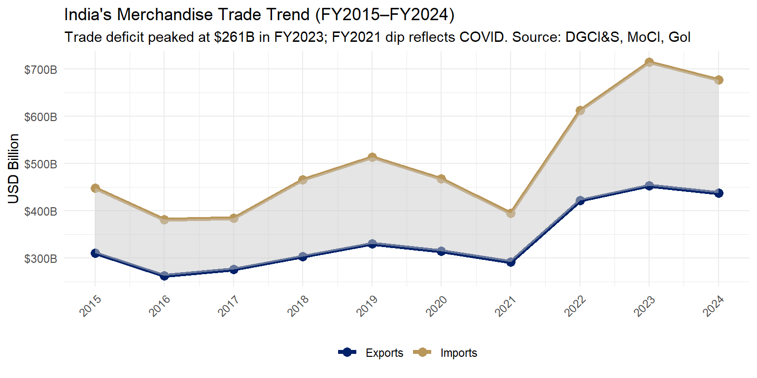
  year    = 2015:2024,
  exports = c(310.3, 262.3, 275.8, 303.5, 330.1, 314.3, 291.8, 422.0, 453.0, 437.1),
  imports = c(448.0, 381.0, 384.4, 465.6, 514.0, 467.2, 394.4, 612.0, 714.2, 677.2)
)
trade_long <- tidyr::pivot_longer(trade_data, cols=c(exports, imports), names_to="type", values_to="value")
trade_long$type <- factor(trade_long$type, levels=c("exports","imports"), 
                           labels=c("Exports","Imports"))

ggplot(trade_long, aes(x=year, y=value, color=type, group=type)) +
  geom_line(linewidth=1.5) +
  geom_point(size=3) +
  geom_ribbon(data=trade_data, aes(x=year, ymin=exports, ymax=imports), 
              inherit.aes=FALSE, fill="grey80", alpha=0.5) +
  scale_color_manual(values=c("Exports"="#012169", "Imports"="#B9975B")) +
  scale_x_continuous(breaks=2015:2024) +
  scale_y_continuous(labels=scales::dollar_format(suffix="B")) +
  labs(title="India's Merchandise Trade Trend (FY2015–FY2024)",
       subtitle="Trade deficit peaked at $261B in FY2023; FY2021 dip reflects COVID. Source: DGCI&S, MoCI, GoI",
       x=NULL, y="USD Billion", color=NULL) +
  theme_minimal(base_size=11) +
  theme(legend.position="bottom", axis.text.x=element_text(angle=45, hjust=1))

Figure 1: India’s Merchandise Trade (FY2015–FY2024, USD billion) Source: DGCI&S / Ministry of Commerce and Industry (GoI).

Key insight: India’s trade deficit widened sharply post-2020, peaking at ~$261B in FY2023. FY2021 saw a COVID-induced contraction (exports fell to $292B). FY2024 saw partial correction: exports $437B, imports $677B — deficit mainly driven by crude oil, gold, and electronics.

India’s Agricultural Trade: FY2024

Top agricultural exports and imports

Commodity (Exports)	Value (USD bn)	Commodity (Imports)	Value (USD bn)
Rice (Basmati + Non-Basmati)	10.4	Edible oils (palm, soy)	14.2
Marine products	7.4	Pulses	3.0
Spices	4.0	Cashew (raw)	1.8
Buffalo meat	3.5	Fresh fruits	1.5
Sugar	2.1	Spices (select)	0.8
Total agri exports	~43.7	Total agri imports	~28.2

Agricultural trade surplus: ~$15.5 billion

Source: APEDA / DGCI&S, 2024

India’s Agricultural Trade Profile

library(ggplot2)

agri_data <- data.frame(
  commodity = c("Rice (Basmati)", "Rice (Non-Basmati)", "Marine Products",
                "Spices", "Sugar", "Cotton", "Other Cereals", "Processed Food",
                "Fruits & Veg", "Oil Meals"),
  value = c(5.8, 4.6, 7.4, 4.0, 2.1, 2.7, 1.9, 4.8, 3.9, 3.5)
)
agri_data <- agri_data |> arrange(value) |>
  mutate(commodity=factor(commodity, levels=commodity))

ggplot(agri_data, aes(x=commodity, y=value)) +
  geom_col(fill="#012169", width=0.7) +
  geom_text(aes(label=paste0("$", value, "B")), hjust=-0.1, size=3.2) +
  coord_flip() +
  labs(title="India's Agricultural Exports, FY2024",
       subtitle="Total: ~$43.7 billion | Rice + Marine dominate",
       x=NULL, y="USD Billion") +
  scale_y_continuous(limits=c(0,9)) +
  theme_minimal(base_size=11)

Figure 2: India’s Agricultural Exports by Commodity, FY2024 (USD billion) Source: APEDA Annual Report 2023–24.

Agriculture’s Share in India’s Trade

Export side

• Agriculture: ~10% of total merchandise exports ($43.7B of $437B)
• Engineering goods: ~26% | Petroleum products: ~17% | Gems & jewellery: ~10%
• Agriculture is India’s second-largest net foreign exchange earner after services
• India’s strengths: rice, spices, marine products, cotton — all labour-intensive, climate-favoured commodities

Import side

• Edible oils: India imports 60–65% of its edible oil requirement (palm, soybean, sunflower)
• Pulses: Canada, Australia, Myanmar — ~25% of domestic requirement imported

Vulnerability: India’s dependence on imported edible oils (~$14B/yr) exposes food inflation to global price shocks, as seen in 2021–22 when palm oil prices spiked 50%.

India’s Position in Global Agricultural Trade

library(ggplot2)

global_share <- data.frame(
  country = c("USA", "Netherlands", "Brazil", "Germany", "France", "China", "India", "Argentina"),
  share = c(11.0, 6.5, 6.3, 5.1, 4.8, 4.5, 2.8, 2.5)
)
global_share <- global_share |> arrange(share) |>
  mutate(country=factor(country, levels=country),
         highlight=ifelse(country=="India", "India", "Others"))

ggplot(global_share, aes(x=country, y=share, fill=highlight)) +
  geom_col(width=0.7) +
  scale_fill_manual(values=c("India"="#B9975B", "Others"="#cccccc")) +
  coord_flip() +
  labs(title="Top Agricultural Exporters: Global Market Share (%)",
       x=NULL, y="Share of World Agricultural Exports (%)", fill=NULL) +
  theme_minimal(base_size=11) +
  theme(legend.position="none") +
  geom_text(aes(label=paste0(share, "%")), hjust=-0.1, size=3.2)

Figure 3: Major Agricultural Exporters: Global Market Share (2023) Source: WTO, World Agricultural Trade Statistics 2024.

India holds 2.8% of world agricultural exports — 7th globally — but punches below its weight given its agricultural size. Significant scope to expand market share in rice, spices, and processed foods.

Key Concepts: Theory

Classical trade theory

• Comparative advantage — trade based on relative, not absolute, efficiency (Ricardo)
• Factor endowments — land, labour, capital abundance shapes what countries export (Heckscher-Ohlin)
• Terms of trade — ratio of export prices to import prices; determines gains from trade
• Intra-industry trade — two-way trade in similar products (India exports basmati, imports parboiled rice)

Comparative advantage explains what countries trade; terms of trade determine how much they gain.

Key Concepts: Policy

Trade policy instruments

• Tariff — tax on imports; raises domestic price above world price
• Non-Tariff Barrier (NTB) — quotas, SPS standards, licensing
• Balance of Payments (BoP) — accounting of all international transactions
• Exchange rate — price of one currency in terms of another; stronger rupee makes exports costlier

Tariffs and NTBs determine how much trade actually occurs — constraining the gains that comparative advantage would otherwise deliver.

Why Study International Trade?

Policy relevance for India

• Foreign Trade Policy 2023–28 targets $2 trillion in merchandise + services exports by 2030
• WTO commitments constrain India’s ability to protect domestic agriculture (AMS limits; tariff bindings)
• Farmer income — ~50% of India’s workforce in agriculture; export markets expand income
• Food security — import policy on pulses and oilseeds directly affects 1.4 billion people

• Academic relevance — Fastest-growing sub-field in development economics; links to climate change, gender, and technology
• Bottom line: International trade policy is agricultural policy in India. They cannot be studied in isolation.

What Makes Agricultural Trade Special?

Biological & physical features

• Perishability — fresh produce, milk, meat have short shelf-lives → need cold chains, quick clearance
• Seasonality — harvests are discrete events; supply is lumpy
• Bulkiness — grain, sugar, cotton: high weight-to-value ratio → high freight costs
• Sanitary risks — food-borne pathogens cross borders with commodities → SPS measures justified

Economic & political features

• Food security concern — governments intervene to ensure domestic supply; export bans, import duty waivers are common
• WTO special treatment — Agreement on Agriculture has Special and Differential Treatment for developing countries

Additional economic/political features: - Price volatility — weather, pests, and speculation create large price swings; farmers and consumers are both affected - Political economy — large farm lobbies in US, EU, India influence trade policy disproportionately

India’s Export Destinations (FY2024)

Top merchandise export destinations

Rank	Country	Share of exports	Key agri exports
1	United States	~18%	Marine, spices
2	UAE	~6.5%	Rice, meat, fruits
3	Netherlands	~4.2%	Spices, cotton
4	China	~3.8%	Cotton, castor oil
5	Bangladesh	~3.5%	Rice, onion, sugar

Gravity model logic: India trades most with large (USA, China) or geographically close (UAE, Bangladesh) economies — a pattern we will formalise in Lecture 2.

India’s Import Sources (FY2024)

Top merchandise import sources

Rank	Country	Share of imports	Key agri imports
1	China	~15%	Electronics, chemicals
2	UAE	~7.5%	Crude oil, gold
3	USA	~6.2%	Pulses, capital goods
4	Russia	~5.8%	Crude oil, fertilisers
5	Saudi Arabia	~5.4%	Crude oil, edible oils

Composition of India’s Merchandise Exports

Major export categories (FY2024, approx.)

Category	Value (USD bn)	Share
Engineering goods	112	25.6%
Petroleum products	78	17.8%
Gems & jewellery	44	10.1%
Chemicals	36	8.2%
Agriculture & allied	44	10.1%
Textiles & apparel	35	8.0%
Electronic goods	29	6.6%

• Engineering goods grew from 12% (2000) to 26% (2024)
• Agriculture has held a stable ~10–12% share for two decades

• Electronic goods rising fast (mobile phones, semiconductors policy)
• India’s export ambition: move up the value chain from raw agri commodities to processed food products

Foreign Trade Policy 2023-28: Five Pillars

Foreign Trade Policy (FTP) 2023–28: Key pillars

1. Export target: $2 trillion merchandise + services exports by 2030
2. Districts as Export Hubs (DEH): Identify 1 product per district with export potential; provide targeted support
3. ECGC coverage: Expanded Export Credit Guarantee Corporation cover to de-risk exporters, especially MSMEs
4. Remission of Duties and Taxes on Exported Products (RoDTEP): Replace old MEIS; neutralise embedded taxes
5. E-commerce exports: Dedicated policy for cross-border e-commerce; target $200–300B by 2030

FTP 2023-28: Agriculture-Specific Provisions

Agricultural trade–specific provisions

• Agri-specific chapters supporting APEDA-registered exporters
• GI tag promotion (Darjeeling tea, Alphonso mangoes, Basmati rice)
• Simplification of phytosanitary certification processes

FTP 2023–28 is notably continuity-oriented — it builds on previous policy architecture rather than a radical overhaul, reflecting India’s cautious approach to trade liberalisation.

A Preview: The Basic Trade Model (I)

PPF — conceptual preview

Without trade (autarky)

• A country produces and consumes on its PPF
• The slope of the PPF = the domestic relative price
• Example: India producing only rice and wheat — the trade-off is fixed by domestic technology

A Preview: The Basic Trade Model (II)

With trade (open economy)

• World price ratio differs from domestic price ratio
• Country specialises in the good where it has comparative advantage
• Consumption point can now lie outside the PPF — both countries gain

Core result: Trade allows a country to consume beyond its production possibilities — through specialisation and exchange.

Upcoming lectures formalise: why world price differs (Lec 3–5), how much each country gains (Lec 7), what tariffs do (Lec 8).

Key Definitions (I)

Trade flows

• Exports — goods/services sold to foreign residents; flow of goods out, money in
• Imports — goods/services bought from foreign residents; flow of goods in, money out
• Trade balance = Exports − Imports (positive → surplus; negative → deficit)
• Visible trade — physical merchandise (rice, cars, oil)
• Invisible trade — services, remittances, investment income

Key Definitions (II)

Balance of Payments

• Current account — trade in goods + services + remittances + investment income
• Capital account — financial flows: FDI, portfolio investment, loans
• BoP identity: Current account + Capital account = 0 (approximately)

Exchange rate

• Nominal exchange rate — ₹/USD; e.g., ₹83 = $1
• Real exchange rate — adjusts for price level differences; determines actual competitiveness

Summary: Why International Trade Matters

Four reasons international trade is essential for India

1. Growth engine: Trade has been central to every development success story — Japan, South Korea, China, and now India’s IT sector

2. Consumer welfare: Trade gives 1.4 billion Indians access to goods they cannot produce cheaply at home

3. Farmer incomes: Export markets for rice, spices, and marine products support millions of rural households

4. Policy discipline: WTO commitments create external pressure for domestic policy reform

India’s challenge: Integrating deeply into global value chains while protecting food security and farm incomes — the central tension this course will explore.

Key Takeaways: Lecture 1

What we covered today

• International trade = cross-border exchange of goods, services, and capital
• Global merchandise trade: ~$25 trillion (2023); services: ~$7 trillion
• India ranks 18th in merchandise exports; total trade ~$1.18 trillion (FY2024)
• Agricultural exports: $43.7 billion (FY2024) — rice, marine, spices, cotton dominate
• India has a structural agricultural trade surplus (~$15.5B) that helps offset the merchandise deficit

• Agricultural trade is special: perishability, food security, seasonality, and political economy all matter
• FTP 2023–28 targets $2 trillion in exports — an ambitious but achievable goal

Questions to think about before next lecture:

1. Why does India ban rice exports during domestic inflation? Who benefits, who loses?
2. If India has absolute advantage in producing rice, why does Bangladesh also export rice?

Next Lecture: Lecture 2

Features of International Trade (May 5, 2026)

We will cover:

• Salient features of international trade that distinguish it from domestic trade
• Immobility of factors — why labour and capital don’t flow freely across borders
• Currency and exchange risk — how rupee movements affect export competitiveness
• Internal vs international trade — a systematic comparison
• The gravity model — intuition and India examples

Also covered: - Advantages and disadvantages of trade — with India-specific examples - India’s edible oil import dependence — a case study in vulnerability

Suggested reading

• Krugman, Obstfeld & Melitz, International Economics, Ch. 1
• APEDA Annual Report 2023–24 (summary statistics)
• FTP 2023–28, Chapter 1 (overview)

Data to explore

• DGCI&S trade statistics (commerce.gov.in)
• WTO Statistics Portal

Appendix

Additional Resources

Further Reading

• International Economics — Salvatore (Ch. 1)
• International Economics — Appleyard & Field (Ch. 1)
• RBI/DGCI&S/APEDA databases for latest data

Key Data Sources

• DGCI&S: India’s merchandise trade
• RBI: Balance of payments data
  
• APEDA: Agricultural export statistics
• WTO: Tariff and trade databases